Apache Kafka®️ 비용 절감 방법 및 최적의 비용 설계 안내 웨비나 | 자세히 알아보려면 지금 등록하세요
KSQL in Football: FIFA Women’s World Cup Data Analysis
One of the football (as per European terminology) highlights of the summer is the FIFA Women’s World Cup. France, Brazil, and the USA are the favourites, and this year Italy is present at the event for the first time in 20 years.
From a data perspective, the World Cup represents an interesting source of information. There’s a lot of dedicated press coverage, as well as the standard social media excitement following any kind of big event.
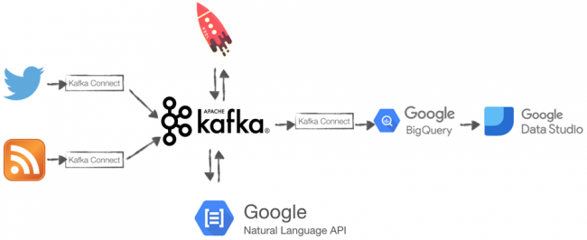
The idea in this blog post is to mix information coming from two distinct channels: the RSS feeds of sport-related newspapers and Twitter feeds of the FIFA Women’s World Cup. The goal will be to understand how the sentiment of official news related to two of the teams involved compares to that of the tweets.
In order to achieve our targets, we’ll use pre-built connectors available in Confluent Hub to source data from RSS and Twitter feeds, KSQL to apply the necessary transformations and analytics, Google’s Natural Language API for sentiment scoring, Google BigQuery for data storage, and Google Data Studio for visual analytics.
Data sources
The beginning of our journey starts with connecting to various data sources. Twitter represents the default source for most event streaming examples, and it’s particularly useful in our case because it contains high-volume event streaming data with easily identifiable keywords that can be used to filter for relevant topics.
Ingesting Twitter data
Ingesting Twitter data is very easy with Kafka Connect, a framework for connecting Kafka with external systems. Within the pre-built connectors, we can find Kafka Connect Twitter; all we need to do is install it using the Confluent Hub client.
confluent-hub install jcustenborder/kafka-connect-twitter:latest
To start ingesting the Twitter data, we need to create a configuration file containing the following important bits:
- filter.keywords: We need to list all the keywords we are interested in, separated by a comma. Since we want to check tweets from the FIFA Women’s World Cup, we’ll use FIFAWWC, representing both the World Cup Twitter handle and the most common related hashtag.
- kafka.status.topic: This is the topic that will be used to store the tweets we selected. We used the topic name twitter_avro since the connector output format is AVRO.
- twitter.oauth: This represents Twitter credentials. More information can be found on the Twitter’s developer website.
After the changes, our configuration file looks like the following:
filter.keywords=FIFAWWC
kafka.status.topic=twitter_avro
twitter.oauth.accessToken=<TWITTER ACCESS TOKEN>
twitter.oauth.accessTokenSecret=<TWITTER ACCESS TOKEN SECRET>
twitter.oauth.consumerKey=<TWITTER ACCESS CUSTOMER KEY>
twitter.oauth.consumerSecret=<TWITTER CUSTOMER SECRET>
It’s time to start it up! We can use the Confluent CLI load command:
confluent local load twitter -- -d $TWITTER_HOME/twitter.properties
$TWITTER_HOME is the folder containing the configuration file. We can check the Kafka Connect status by querying the REST APIs with the following:
curl -s "http://localhost:8083/connectors/twitter/status" | jq [.connector.state]
We can also check if all the settings are correct by consuming the AVRO messages in the twitter_avro topic with a console consumer:
confluent local consume twitter_avro -- --value-format avro
And the result is, as expected, an event stream of tweets.

RSS feeds as another data source
The second data source that we’ll use for our FIFA Women’s World Cup sentiment analytics are RSS feeds from sports-related newspapers. RSS feeds are useful because they share official information about teams and players, like results, episodes, and injuries. RSS feeds should be considered neutral since they should only report facts. For this blog post, we’ll use RSS feeds as a way to measure the average sentiment of the news. As per the Twitter case above, a prebuilt Kafka Connect RSS Source exists, so all we need to do is to install it via the Confluent Hub client:
confluent-hub install kaliy/kafka-connect-rss:latest
Then, create a configuration file with the following important parameters:
- rss.urls: This is a list of space-separated RSS feed URLs. For our Women’s World Cup example, we’ve chosen the following sources:
- La Gazzetta dello Sport
- Transfermarkt
- Eurosport
- UEFA
- The Guardian
- Daily Mail
- The Sun Daily
- BBC
- topic: The Kafka topic to write to, which is rss_avro in our case
The full configuration file looks like the following:
name=RssSourceConnector
tasks.max=1
connector.class=org.kaliy.kafka.connect.rss.RssSourceConnector
rss.urls=https://www.transfermarkt.co.uk/rss/news https://www.eurosport.fr/rss.xml https://www.uefa.com/rssfeed/news/rss.xml https://www.theguardian.com/football/rss https://www.dailymail.co.uk/sport/index.rss https://www.thesundaily.my/rss/sport http://feeds.bbci.co.uk/news/rss.xml https://www.gazzetta.it/rss/home.xml
topic=rss_avro
And again, we can start the ingestion of RSS feeds with the Confluent CLI:
confluent local load RssSourceConnector -- -d $RSS_HOME/RssSourceConnector.properties
We can test the status of the Kafka Connect RssSourceConnector using this simple procedure and calling it:
./connect_status.sh
RssSourceConnector  |  RUNNING  |  RUNNING
twitter             |  RUNNING  |  RUNNING
We can see that the both the RssSourceConnector and the twitter Connect are up and running. We can then check the actual data with the console consumer:
confluent local consume rss_avro -- --value-format avro
Below is the output as expected.

Shaping the event streams
After ingesting the Twitter and RSS event streams into topics, it’s time to shape them with KSQL. Shaping the topics accomplishes two purposes:
- It makes the topics queryable from KSQL
- It defines additional structures that can be reused in downstream applications
The Twitter stream lands in Avro format with the fields listed in the related GitHub repo. We can easily declare a TWITTER_STREAM KSQL stream on top of TWITTER_AVRO with:
CREATE STREAM TWITTER_STREAM WITH (
    KAFKA_TOPIC='TWITTER_AVRO',
    VALUE_FORMAT='AVRO',
    TIMESTAMP='CREATEDAT'
    );
There is no need to define the single fields in the event stream declaration because they are already in AVRO and thus will be sourced from the Confluent Schema Registry. Schema Registry is the component within Kafka, in charge of storing, versioning and serving the topics Avro Schemas. When a topic is in AVRO format, its schema is stored in the Schema Registry, where downstream applications (like KSQL in this case) can retrieve it and use it to “shape” the messages in the topic.
The important bits of the above KSQL for our definition are:
- KAFKA_TOPIC='TWITTER_AVRO': the definition of the source topic
- VALUE_FORMAT='AVRO': the definition of the source topic format
- TIMESTAMP='CREATEDAT': the Tweet’s creation date, which is used as the event timestamp
We can now check that the fields’ definition has correctly been retrieved by the Schema Registry with:
DESCRIBE TWITTER_STREAM;
Or, we can use the REST API by:
curl -X "POST" "http://localhost:8088/ksql" \
     -H "Content-Type: application/vnd.ksql.v1+json; charset=utf-8" \
     -d $'{
  "ksql": "DESCRIBE TWITTER_STREAM;",
  "streamsProperties": {}
}'
The resulting fields section will be:
"fields": [
        {
          "name": "ROWTIME",
          "schema": {
            "type": "BIGINT",
            "fields": null,
            "memberSchema": null
    },
    {
      "name": "ROWKEY",
      "schema": {
        "type": "STRING",
        "fields": null,
        "memberSchema": null

    },
    {
      "name": "CREATEDAT",
      "schema": {
        "type": "BIGINT",
        "fields": null,
        "memberSchema": null

    },
    {
      "name": "ID",
      "schema": {
        "type": "BIGINT",
        "fields": null,
        "memberSchema": null

    },
... }
The same applies to the RSS feed contained in rss_avro with:
create stream RSS_STREAM
WITH(
KAFKA_topic='rss_avro',
TIMESTAMP='DATE',
TIMESTAMP_FORMAT='yyyy-MM-dd''T''HH:mm:ss''Z''',
VALUE_FORMAT='AVRO'
)
The result will be:
Name                 : RSS_STREAM
 Field   | Type
--------------------------------------------------------------
 ROWTIME | BIGINT           (system)
 ROWKEY  | VARCHAR(STRING)  (system)
 FEED    | STRUCT
 TITLE   | VARCHAR (STRING)
 ID      | VARCHAR (STRING)
 LINK    | VARCHAR (STRING)
 CONTENT | VARCHAR (STRING)
 AUTHOR  | VARCHAR (STRING)
 DATE    | VARCHAR (STRING)
--------------------------------------------------------------
We can also use the URL manipulation functions added in KSQL 5.2 to extract useful information from the LINK column with:
CREATE STREAM RSS_STREAM_URL_DECODING AS
SELECT LINK,
  URL_EXTRACT_HOST(LINK) HOST,
  URL_EXTRACT_PATH(LINK) PATH,
  URL_EXTRACT_PROTOCOL(LINK) PROTOCOL,
  URL_EXTRACT_QUERY(LINK) QUERY_TEXT
FROM RSS_STREAM;
The result will be:
ksql> SELECT HOST, PATH, PROTOCOL, QUERY_TXT FROM RSS_STREAM_URL_DECODING LIMIT 5;
www.dailymail.co.uk | /sport/football/article-6919585/Paul-Scholes-backs-Manchester-United-spring-surprise-Barcelona.html | https | ns_mchannel=rss&ns_campaign=1490&ito=1490
www.dailymail.co.uk | /sport/formulaone/article-6916337/Chinese-Grand-Prix-F1-race-LIVE-Shanghai-International-Circuit.html | https | ns_mchannel=rss&ns_campaign=1490&ito=1490
www.dailymail.co.uk | /sport/football/article-6919403/West-Brom-make-approach-Preston-manager-Alex-Neil.html | https | ns_mchannel=rss&ns_campaign=1490&ito=1490
www.dailymail.co.uk | /sport/football/article-6919373/Danny-Murphy-Jermaine-Jenas-fascinating-mind-games-thrilling-title-race.html | https | ns_mchannel=rss&ns_campaign=1490&ito=1490
www.dailymail.co.uk | /sport/football/article-6919215/Brazilian-legend-Pele-successfully-undergoes-surgery-remove-kidney-stone-Sao-Paulo-hospital.html | https | ns_mchannel=rss&ns_campaign=1490&ito=1490
Limit Reached
Query terminated
Sentiment analytics and Google’s Natural Language APIs
Text processing is a part of machine learning and is continuously evolving with a huge variety of techniques and related implementations. Sentiment analysis represents a branch of text analytics and aims to identify and quantify affective states contained in a text corpus.
Natural Language APIs provide sentiment scoring as a service using two dimensions:
- Score: Positive (Score > 0) or Negative (Score < 0) Emotion
- Magnitude: Emotional Content Amount
For more information about sentiment score and magnitude interpretation, refer to the documentation.
Using Natural Language APIs presents various benefits:
- Model training: Natural Language is a pre-trained model, ideal in situations where we don’t have a set of already-scored corpuses.
- Multi-language: RSS feeds and tweets can be written in multiple languages. Google Natural Language is capable of scoring several languages natively.
- API call: Natural Language can be called via an API, making the integration easy with other tools.
Sentiment scoring in KSQL with user- defined functions (UDFs)
The Natural Language APIs are available via client libraries in various languages, including Python, C#, and Go. For the purposes of this blog post, we’ll be looking at the Java implementation since it is currently the language used to implement KSQL user-defined functions (UDFs). For more details on how to build a UD(A)F function, please refer to How to Build a UDF and/or UDAF in KSQL 5.0 by Kai Waehner, which we’ll use as base for the GSentiment class definition.
The basic steps to implementing Natural Language API calls in a UDF are the following:
- Add the google.cloud.language JAR dependency in your project. If you are using Maven, you just need to add the following in your pom.xml <dependency>:
<dependency> <groupId>com.google.cloud</groupId><artifactId>google-cloud-language</artifactId> <version>1.25.0</version></dependency>
- Create a new Java class called GSentiment.
- Import the required classes:
//KSQL UDF Classes import io.confluent.ksql.function.udf.Udf; import io.confluent.ksql.function.udf.UdfDescription; //Google NL Classes import com.google.cloud.language.v1.LanguageServiceClient; import com.google.cloud.language.v1.Sentiment; import com.google.cloud.language.v1.AnalyzeSentimentResponse; import com.google.cloud.language.v1.Document; import com.google.cloud.language.v1.Document.Type;
- Define the GSentiment class and add the Java annotations:
@UdfDescription(name = "gsentiment", description = "Sentiment scoring using Google NL API") public class Gsentiment { ... } - Within the class, declare gsentiment as the method accepting a String text as input. As of now, UDFs can’t return two output values, so we are returning the sentiment score and magnitude as an array of double.
@Udf(description = "return sentiment scoring") public List gsentiment( String text) { ... } - Within the gsentiment method, invoke the Natural Language API sentiment and cast the result as an array. Since a UDF can return only one parameter currently, we need to pipe the sentiment score and magnitude into an array of two elements.
Double[] arr = new Double[2]; try (LanguageServiceClient languageServiceClient = LanguageServiceClient.create()) { Document document = Document.newBuilder() .setContent(text) .setType(Type.PLAIN_TEXT) .build(); AnalyzeSentimentResponse response = languageServiceClient.analyzeSentiment(document); Sentiment sentiment = response.getDocumentSentiment();arr[0]=(double)sentiment.getMagnitude(); arr[1]=(double)sentiment.getScore(); } catch (Exception e) { arr[0]=(double) 0.0; arr[1]=(double) 0.0; } return Arrays.asList(arr);
- As mentioned in How to Build a UDF and/or UDAF in KSQL 5.0, build an uber JAR that includes the KSQL UDF and any dependencies, and copy it to the KSQL extension directory (defined in the ksql.extension.dir parameter in ksql-server.properties).
- Add an environment variable GOOGLE_APPLICATION_CREDENTIALS pointing to the service account key that will be used to authenticate to Google services.
- Restart KSQL.
- topics: defines the topic to read (in our case RSS_STREAM_WITH_SENTIMENT_DETAILS and TWITTER_STREAM_WITH_SENTIMENT_DETAILS)
- project: the name of the Google project that we’ll use for billing
- datasets=.*=wwc: defines the BigQuery dataset name
- keyfile=$GOOGLE_CRED/myGoogleCredentials.json: points to the JSON file containing Google’s credentials (which in our case is the same file used in the Google Natural Language scoring)
- Download the Confluent Platform to get started with the leading distribution of Apache Kafka
- Learn about ksqlDB, the successor to KSQL, and see the latest syntax
- Rittman Mead also provides a 30-day Kafka quick start package
At this point, we should be able to call the GSentiment UDF from KSQL:
ksql> SELECT GSENTIMENT(text) FROM TWITTER_STREAM LIMIT 5;
[0.10000000149011612, -0.10000000149011612]
[0.20000000298023224, 0.20000000298023224]
[0.5, 0.10000000149011612]
[0.10000000149011612, 0.10000000149011612]
[0.0, 0.0]
Limit Reached
Query terminated
As expected, the UDF returns an ARRAY of numbers. In order to get the sentiment score and magnitude in separated columns, we simply need to extract the relevant values:
ksql> SELECT GSENTIMENT(TEXT)[0] SCORE, GSENTIMENT(TEXT)[1] MAGNITUDE FROM TWITTER_STREAM LIMIT 5;
0.20000000298023224 | 0.10000000149011612
0.30000001192092896 | 0.10000000149011612
0.800000011920929 | 0.800000011920929
0.0 | 0.0
0.30000001192092896 | 0.30000001192092896
Limit Reached
Query terminated
However, we should note that Natural Language APIs are priced per API call and, in the above SQL, we are calling the API two times—one for each GSENTIMENT call. Therefore, the above SQL will cost us two API calls per document. To optimise the cost, we can create a new event stream TWITTER_STREAM_WITH_SENTIMENT, which will physicalize in Kafka the array.
CREATE STREAM TWITTER_STREAM_WITH_SENTIMENT AS
SELECT
    *,
    GSENTIMENT(TEXT) AS SENTIMENT
FROM TWITTER_STREAM;
Next, parse the sentiment SCORE and MAGNITUDE from the TWITTER_STREAM_WITH_SENTIMENT event stream:
CREATE STREAM TWITTER_STREAM_WITH_SENTIMENT_DETAILS as
SELECT *,
    SENTIMENT[0] SCORE,
    SENTIMENT[1] MAGNITUDE
FROM TWITTER_STREAM_WITH_SENTIMENT;
With this second method, we optimize the cost with a single Natural Language API call per tweet. We can do the same with the RSS feeds by declaring:
CREATE STREAM RSS_STREAM_WITH_SENTIMENT AS
SELECT
    *,
    GSENTIMENT(CONTENT) SENTIMENT
FROM RSS_STREAM_FLATTENED;
CREATE STREAM RSS_STREAM_WITH_SENTIMENT_DETAILS as
SELECT *,
    SENTIMENT[0] SCORE,
    SENTIMENT[1] MAGNITUDE
FROM RSS_STREAM_WITH_SENTIMENT;
Sink to Google BigQuery
The following part of this blog post focuses on pushing the dataset into Google BigQuery and visual analysis in Google Data Studio.
Pushing the data into BigQuery is very easy—just install the BigQuery Sink Connector with:
confluent-hub install wepay/kafka-connect-bigquery:latest
Next, configure it while applying the following parameters (amongst others):
Before starting the connector, we need to ensure the BigQuery dataset named wwc (as per configuration file) exists, otherwise, the connector will fail. To do so, we can log into BigQuery, select the same project defined in the configuration file, and click on CREATE DATASET. Then, we’ll need to fill in all the details (more information about the dataset creation in the Google documentation).
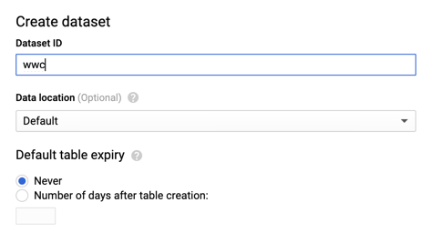
After creating the dataset, it’s time to start the connector with the Confluent CLI:
confluent local load bigquery-connector -- -d $RSS_HOME/connectorBQ.properties
If the Kafka sink works, we should see one table per topic defined in the configuration file, which are RSS_STREAM_WITH_SENTIMENT_DETAILS and TWITTER_STREAM_WITH_SENTIMENT_DETAILS in our case.

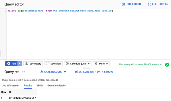
Of course, we can query the data from BigQuery itself.
Visual analysis in Google Data Studio
To start analysing the data in Google Data Studio, simply connect to the related console and select “Blank Report.”
We’ll be asked which data source to use for the project. Thus, we need to set up a connection to the wwc dataset by clicking on CREATE NEW DATASOURCE and selecting BigQuery as the connection. Then, select the project, dataset, and table (TWITTER_STREAM_WITH_SENTIMENT_DETAILS).

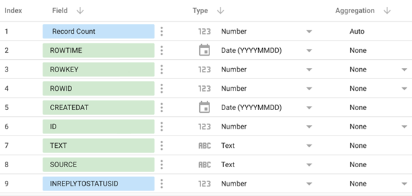
We can then review the list of columns, types, and aggregations, adding the data source to the report.
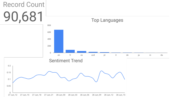
Finally, we can start creating visualisations like tiles to show record counts, line charts for the sentiment trend, and bar charts defining the most used languages.
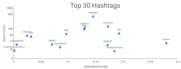
A more advanced visualisation like a scatterplot shows the most common hashtags and the associated average sentiment value.
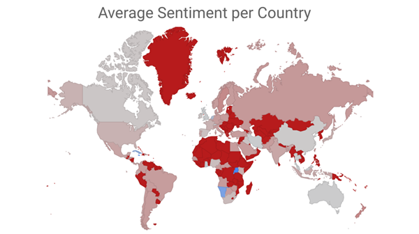
Below is a map visualising the average sentiment by country.
Analysing and comparing sentiment scores
Now that we have the two streams of data coming from Twitter and RSS feeds, we can do the analysis in KSQL and, in parallel, visually in Google Data Studio. We can, for example, examine the average sentiment over a timeframe and check how one source sentiment score compares to the other.
On the 27th of June, the quarterfinal match between Norway and England was played, with the result being that England beat Norway 3–0. Let’s check if we can somehow find significant similarities in the sentiment scoring of our dataset.
Starting with the Twitter feed, we can check all the tweets including ENGLAND and NORWAY by filtering the related hashtag #NORENG. To obtain the team related overall score, I’m then assigning to each team all the tweets containing the country full name and aggregating the SENTIMENTSCORE with the following SQL:
CREATE STREAM TWITTER_NORWAY_ENGLAND AS
SELECT
CASE
       WHEN UCASE(TEXT) LIKE '%NORWAY%' THEN SENTIMENTSCORE
       END AS NORWAY_SENTIMENTSCORE,
CASE
       WHEN UCASE(TEXT) LIKE '%ENGLAND%' THEN SENTIMENTSCORE
       END AS ENGLAND_SENTIMENTSCORE
FROM TWITTER_STREAM_WITH_SENTIMENT_DETAILS
WHERE TEXT LIKE '%#NORENG%';
We can check the overall sentiment score associated with the two teams using:
SELECT
SUM(NORWAY_SENTIMENTSCORE)/COUNT(NORWAY_SENTIMENTSCORE) AS NORWAY_AVG_SCORE,
SUM(ENGLAND_SENTIMENTSCORE)/COUNT(ENGLAND_SENTIMENTSCORE) AS ENGLAND_AVG_SCORE
FROM TWITTER_NORWAY_ENGLAND
GROUP BY 1;
The GROUP BY 1 is necessary since KSQL currently requires a GROUP BY clause when using aggregation functions like SUM. Since we don’t aggregate for any columns other than the window time, we can use the number 1 as fix aggregator for the total. The result of the above query is in line with the final score, with the winner (England) having an average sentiment score of 0.212, and the loser (Norway) having a score of 0.0979.
We can also look at the behaviour per hour with the TUMBLING KSQL windowing function:
SELECT
  TIMESTAMPTOSTRING(WINDOWSTART(), 'EEE dd MMM HH') AS START_WINDOW,
  SUM(NORWAY_SENTIMENTSCORE)/COUNT(NORWAY_SENTIMENTSCORE) AS NORWAY_AVG_SCORE,
  SUM(ENGLAND_SENTIMENTSCORE)/COUNT(ENGLAND_SENTIMENTSCORE) AS ENGLAND_AVG_SCORE
FROM TWITTER_NORWAY_ENGLAND
WINDOW TUMBLING(SIZE 1 HOURS)
GROUP BY 1;
The query yields the following result:
Thu 27 Jun 16 | 0.18409091 | 0.16075758
Thu 27 Jun 17 | 0.14481481 | 0.13887096
Thu 27 Jun 18 | 0.14714406 | 0.12107647
Thu 27 Jun 19 | 0.07926398 | 0.34757579
Thu 27 Jun 20 | 0.10077705 | 0.13762544
Thu 27 Jun 21 | 0.08387538 | 0.17832865
We can clearly see that towards match time (19:00 BST), the ENGLAND average score has a spike coincidentally with England’s first goal in the third minute. We can see the same on the line chart in Google Data Studio.

We can do a similar exercise on top of the RSS feeds stream, but first, we need to somehow filter it to get only FIFA Women’s World Cup 2019 data, since the predefined connector is ingesting all the news from the RSS sources without a topic filter. To do so, we create a new stream filtering only contents containing WOMEN and CUP:
CREATE STREAM RSS_STREAM_WITH_SENTIMENT_DETAILS_WWC as
SELECT *
FROM RSS_STREAM_WITH_SENTIMENT_DETAILS
WHERE UCASE(CONTENT) LIKE '%WOMEN%'
  AND UCASE(CONTENT) LIKE '%CUP%';
We can now analyse the overall RSS sentiment with:
SELECT SUM(SENTIMENTSCORE)/COUNT(SENTIMENTSCORE)
FROM RSS_STREAM_WITH_SENTIMENT_DETAILS_WWC
GROUP BY 1;
As before, the SUM(SENTIMENTSCORE)/COUNT(SENTIMENTSCORE) is calculating the average. We can then calculate the sentiment average for the selected team. Taking the same example of ENGLAND and NORWAY used previously, we just declare a stream filtering the sentiment for the two nations. For example:
CREATE STREAM RSS_NORWAY_ENGLAND AS
SELECT
       CASE WHEN UCASE(CONTENT) LIKE '%NORWAY%' THEN SENTIMENTSCORE END NORWAY_SENTIMENTSCORE,
       CASE WHEN UCASE(CONTENT) LIKE '%ENGLAND%' THEN SENTIMENTSCORE END ENGLAND_SENTIMENTSCORE
FROM RSS_STREAM_WITH_SENTIMENT_DETAILS_WWC;
Then, we can analyse the separate scoring with:
SELECT
      SUM(NORWAY_SENTIMENTSCORE)/COUNT(NORWAY_SENTIMENTSCORE) NORWAY_AVG_SENTIMENT,
      SUM(ENGLAND_SENTIMENTSCORE)/COUNT(ENGLAND_SENTIMENTSCORE) ENGLAND_AVG_SENTIMENT
FROM RSS_NORWAY_ENGLAND
WHERE ROWTIME > STRINGTODATE('2019-06-27', 'yyyy-MM-dd')
GROUP BY 1;
The result is an average sentiment of 0.0575 for Norway and 0.111 for England, again in line with the match result where England won 3–0.
We can also understand the variation of the sentiment over time by using KSQL windowing functions like TUMBLING:
SELECT
  TIMESTAMPTOSTRING(WINDOWSTART(), 'EEE dd MMM HH') START_WINDOW,
  SUM(NORWAY_SENTIMENTSCORE)/COUNT(NORWAY_SENTIMENTSCORE) NORWAY_AVG_SENTIMENT,
  SUM(ENGLAND_SENTIMENTSCORE)/COUNT(ENGLAND_SENTIMENTSCORE) ENGLAND_AVG_SENTIMENT
FROM RSS_NORWAY_ENGLAND WINDOW TUMBLING(SIZE 1 HOURS)
WHERE ROWTIME >= STRINGTODATE('2019-06-27', 'yyyy-MM-dd')
GROUP BY 1;
This yields the following results:
Thu 27 Jun 17 | 0.12876364 | 0.12876364
Thu 27 Jun 18 | 0.24957054 | 0.24957054
Thu 27 Jun 19 | 0.15606978 | 0.15606978
Thu 27 Jun 20 | 0.09970317 | 0.09970317
Thu 27 Jun 21 | 0.00809077 | 0.00809077
Thu 27 Jun 23 | 0.41298701 | 0.12389610
As expected from this source, most of the scoring of the two countries are the same since the number of articles is limited and almost all articles mention both ENGLAND and NORWAY.
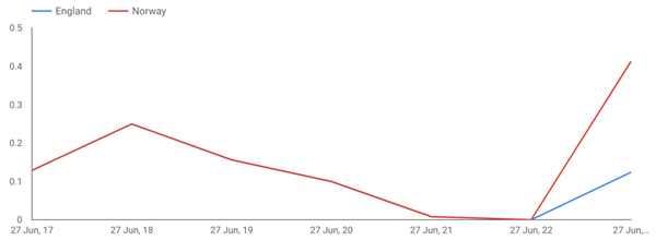
Strangely, as we can see in the graph above, the NORWAY sentiment score on the 27th of June at 11:00 pm GMT (so after the match ended) is much higher than the ENGLAND one.
We can look at the data closely with:
SELECT ROWKEY, NORWAY_SENTIMENTSCORE, ENGLAND_SENTIMENTSCORE
from NORWAY_ENGLAND where TIMESTAMPTOSTRING(ROWTIME,'dd/MM HH') = '27/06 23';
https://www.theguardian.com/...      | 0.375974032  | 0.375974032
https://www.bbc.co.uk/.../48794550   | null         | -0.45428572
https://www.bbc.co.uk/.../48795487   | 0.449999988  | 0.449999988
We can see that NORWAY is being associated with two articles: one from The Guardian with a positive 0.375 score and one from BBC with a positive 0.449 score. ENGLAND, on the other hand, is associated with another BBC article, having a negative -0.454 score.
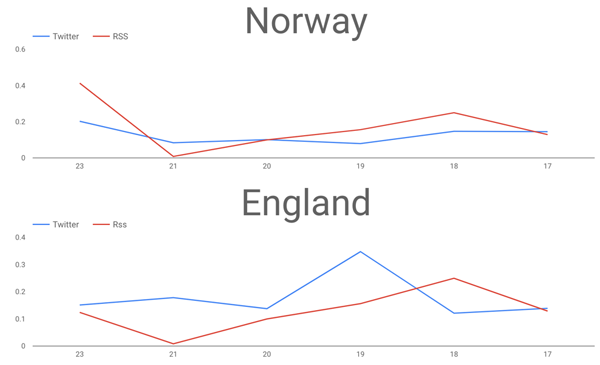
We can also compare the hourly Twitter and RSS sentiment scores by creating two tables:
CREATE TABLE TWITTER_NORWAY_ENGLAND_TABLE AS
SELECT
  TIMESTAMPTOSTRING(WINDOWSTART(), 'dd HH') START_WINDOW,
  SUM(NORWAY_SENTIMENTSCORE)/COUNT(NORWAY_SENTIMENTSCORE) NORWAY_AVG_SCORE,
  SUM(ENGLAND_SENTIMENTSCORE)/COUNT(ENGLAND_SENTIMENTSCORE) ENGLAND_AVG_SCORE
FROM TWITTER_NORWAY_ENGLAND
WINDOW TUMBLING(SIZE 1 HOURS)
GROUP BY 1;
CREATE TABLE RSS_NORWAY_ENGLAND_TABLE AS
SELECT
  TIMESTAMPTOSTRING(WINDOWSTART(), 'dd HH') START_WINDOW,
  SUM(NORWAY_SENTIMENTSCORE)/COUNT(NORWAY_SENTIMENTSCORE) NORWAY_AVG_SCORE,
  SUM(ENGLAND_SENTIMENTSCORE)/COUNT(ENGLAND_SENTIMENTSCORE) ENGLAND_AVG_SCORE
FROM NORWAY_ENGLAND WINDOW TUMBLING(SIZE 1 HOURS)
WHERE ROWTIME >= STRINGTODATE('2019-06-27', 'yyyy-MM-dd')
GROUP BY 1;
The key of both the tables is the window start date, as we can see from:
ksql> select rowkey from RSS_NORWAY_ENGLAND_TABLE limit 1;
1 : Window{start=1561557600000 end=-}
We can then join the results together with the following statement:
SELECT A.START_WINDOW,
  A.NORWAY_AVG_SENTIMENT TWITTER_NORWAY_SCORE,
  A.ENGLAND_AVG_SENTIMENT TWITTER_ENGLAND_SCORE,
  B.NORWAY_AVG_SENTIMENT RSS_NORWAY_SCORE,
  B.ENGLAND_AVG_SENTIMENT RSS_ENGLAND_SCORE
FROM
  TWITTER_NORWAY_ENGLAND_TABLE A JOIN
  RSS_NORWAY_ENGLAND_TABLE B
ON A.ROWKEY = B.ROWKEY;
This yields the following result:
Thu 27 Jun 17 | 0.14481481 | 0.13887096 | 0.12876364 | 0.12876364
Thu 27 Jun 18 | 0.14714406 | 0.12107647 | 0.24957054 | 0.24957054
Thu 27 Jun 19 | 0.07926398 | 0.34757579 | 0.15606978 | 0.15606978
Thu 27 Jun 20 | 0.10077705 | 0.13762544 | 0.09970317 | 0.09970317
Thu 27 Jun 21 | 0.08387538 | 0.17832865 | 0.00809077 | 0.00809077
At the end, the result is similar in a Data Studio line chart.
Interested in more?
이 블로그 게시물이 마음에 드셨나요? 지금 공유해 주세요.
Confluent 블로그 구독
3 Strategies for Achieving Data Efficiency in Modern Organizations
The efficient management of exponentially growing data is achieved with a multipronged approach based around left-shifted (early-in-the-pipeline) governance and stream processing.
Chopped: AI Edition - Building a Meal Planner
Dinnertime with picky toddlers is chaos, so I built an AI-powered meal planner using event-driven multi-agent systems. With Kafka, Flink, and LangChain, agents handle meal planning, syncing preferences, and optimizing grocery lists. This architecture isn’t just for food, it can tackle any workflow.

