[Virtual Event] GenAI Streamposium: Learn to Build & Scale Real-Time GenAI Apps | Register Now
Analysing Historical and Live Data with ksqlDB and Elastic Cloud
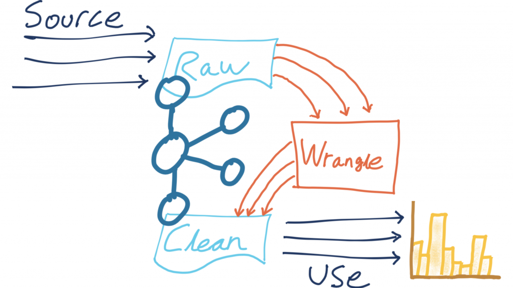
Building data pipelines isn’t always straightforward. The gap between the shiny “hello world” examples of demos and the gritty reality of messy data and imperfect formats is sometimes all too easily glossed over. I want to show you some techniques for bridging this gap. We’re going to take a raw stream of data in Apache Kafka®, smarten it up and make it presentable, and stream it onward to drive an analytics dashboard.
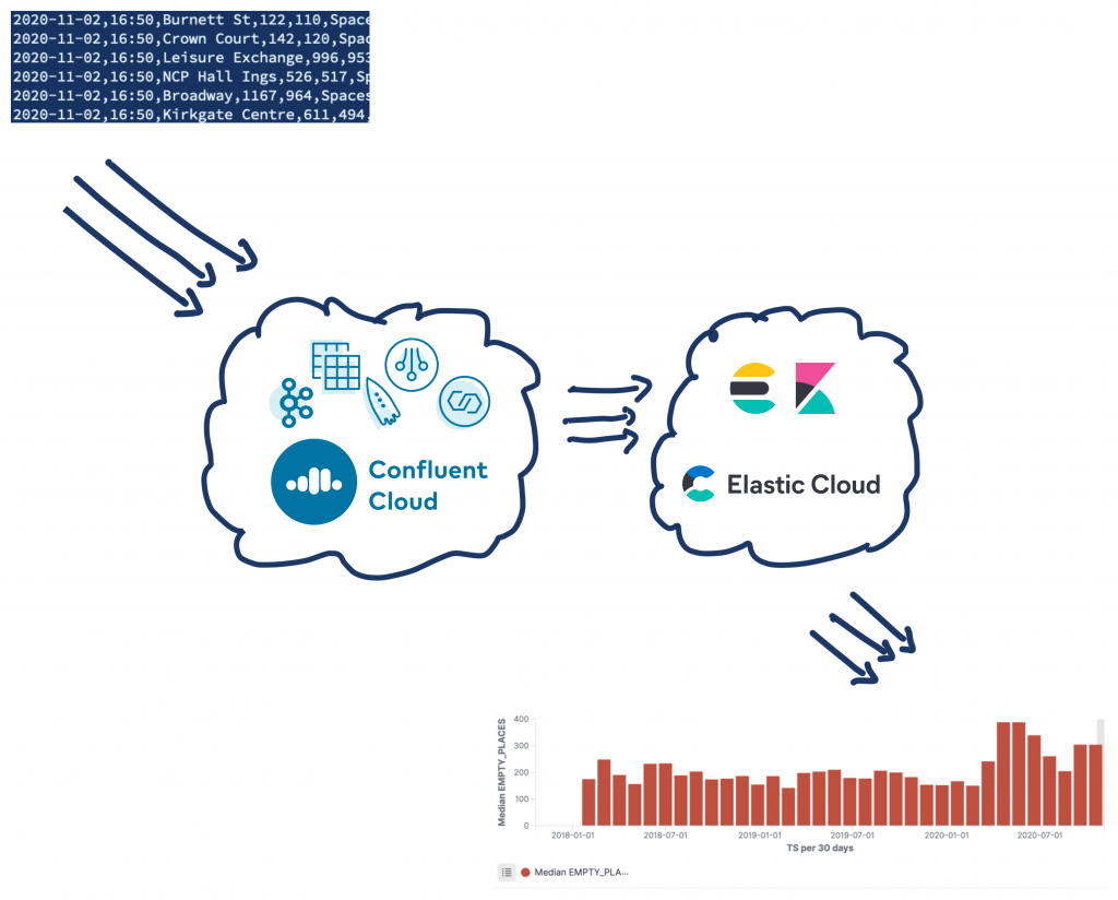
The data comes from the Northern Data Hub and provides information about the occupancy of car parks in the city centre of Bradford, England. Each message is comma separated and looks like this:
2020-10-06,14:41,Westgate,116,89,Spaces,53.796291,-1.759143,"https://maps.google.com/?daddr=53.796291,-1.759143"
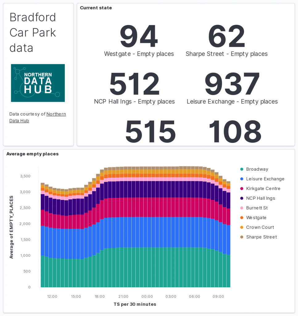
The goal is to transform this data and use it to drive a real-time dashboard. Elasticsearch will be used to store the data and Kibana will be used to visualise it.
Best of all? It’s all done using managed services from Confluent and Elastic, leaving you the time to build pipelines to benefit your business—not spend the time and resources running the underlying hardware and systems. Of course, if you’d rather run it on premises, you can do that too 🙂
What are we going to do to the data?
The source data is in a Kafka topic on Confluent Cloud, and we’re going to use ksqlDB to process events from the source topic as they arrive. We’ll apply the transformations and write the modified event to a target topic. That target topic then becomes the source for streaming data down to Elasticsearch for analytics.
The transformations we’re going to do are:
- Applying and storing a schema for the data
- Setting the message key for partitioning
- Adding a source field for lineage
- Deriving and storing the timestamp in an appropriate data type
- Creating a nested field (struct) to hold the location latitude/longitude pair
- Creating a calculated field
| ℹ️ | I’m using ksqlDB on Confluent Cloud. If you want to try it out use the promo code RMOFF200 when signing up to receive an additional $200 of free usage (see details). |
A schema, a schema…my kingdom for a schema!
The messages that arrive on the Kafka topic are raw CSV data—just a string of values with commas.

If we’re going to do anything with this data, we are going to need to apply a schema to it at some point in order to be able to make sense of it. Otherwise, it’s just a long string. A good pattern to follow is “transform once, use many.” By applying a commonly required transformation to the data (such as a schema) and writing the result back on to a Kafka topic, we—and any other consuming application—can benefit from it.
There are two key reasons to apply a schema to your data early on in its Kafka lifecycle. First, consumers can use the data without needing to find out the schema details from the application team that produced the data (which also would introduce a tight coupling between your systems). Second, the brittleness of pipelines is reduced, as the compatibility of new messages with those on an existing topic can be enforced. This prevents producers from writing messages to the topic that the consumer would not be able to handle.
You can learn more about the importance of schemas here:
- ✍️ Schemas, Contracts, and Compatibility
- ✍️ Yes, Virginia, You Really Do Need a Schema Registry
- 🎥 Streaming Microservices: Contracts and Compatibility – Gwen Shapira – QCon
We use the Confluent Schema Registry to hold the schema, and write the data back onto a new Kafka topic that is serialised using an appropriate format, such as Protobuf, Avro, or JSON Schema.

To start with, we use the CREATE STREAM ksqlDB statement with the schema declared in full and the Kafka topic to which to apply it:
CREATE STREAM CARPARK_SRC (date          VARCHAR ,
                           time          VARCHAR ,
                           name          VARCHAR ,
                           capacity      INT ,
                           empty_places  INT ,
                           status        VARCHAR ,
                           latitude      DOUBLE ,
                           longitude     DOUBLE ,
                           directionsURL VARCHAR)
                WITH (KAFKA_TOPIC='carparks',
                      VALUE_FORMAT='DELIMITED');
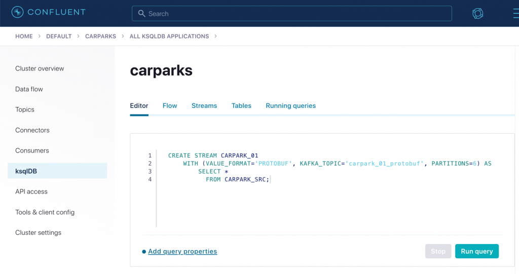
To serialise this to a new topic and store the schema in the Schema Registry, we use CREATE STREAM again. This time, it’s CREATE STREAM…AS SELECT, which writes the continual output of the declared SELECT into a target Kafka topic:
CREATE STREAM CARPARK_01
    WITH (VALUE_FORMAT='PROTOBUF', KAFKA_TOPIC='carpark_01_protobuf', PARTITIONS=6) AS
    SELECT *
      FROM CARPARK_SRC;
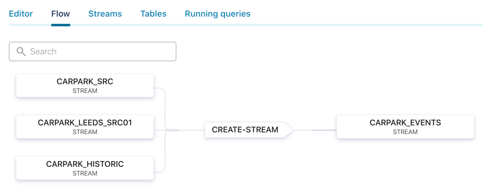
ksqlDB provides a helpful visualisation of your data flow:
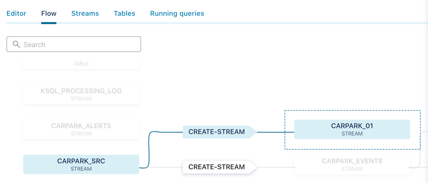
It also offers a preview of the messages as they flow through:
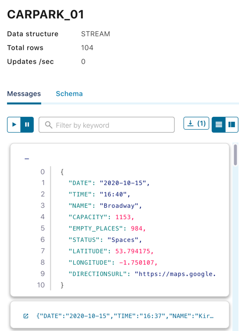
Apply a message key
The producing application that writes the data to our source topic, carparks, does not—for whatever reason—set the message key. This means that data for any car park can end up on any partition – which is not necessarily what we want. We can build on the above CREATE STREAM statement to also apply a partitioning key of the name of the car park to the resulting messages.
CREATE STREAM EXAMPLE_02 AS
    SELECT *
      FROM CARPARK_01
    PARTITION BY NAME;
Because Kafka stores data for as long as we configure it to (on a per-topic basis), we can run these stream processing transformations against not only the new messages as they arrive on the source topic but also all the existing messages already on the topic. To do this, we set the offset from which ksqlDB will process back to earliest (by default, it’s latest, processing only new messages):
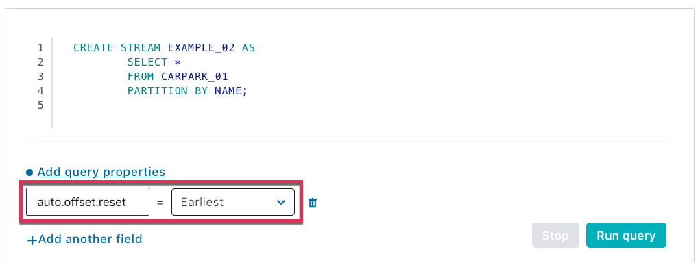
If you’re doing this from the ksqlDB CLI, then issue a SET command:
ksql> SET 'auto.offset.reset' = 'earliest';
| ℹ️ | Psst if you want to check for yourself that the messages now have the key set correctly, you can use a tool like kafkacat to do this: |
# Set your Confluent Cloud details in the environment variables
# used here
docker run --rm --interactive edenhill/kafkacat:1.6.0 \
-b $CCLOUD_BROKER_HOST -X sasl.username="$CCLOUD_API_KEY" -X sasl.password="$CCLOUD_API_SECRET" -X security.protocol=SASL_SSL -X sasl.mechanisms=PLAIN -X ssl.ca.location=./etc/ssl/cert.pem -X api.version.request=true \
-t EXAMPLE_02 -C -J | jq '.'
{
"topic": "EXAMPLE_02",
"partition": 3,
"offset": 4742,
"tstype": "create",
"ts": 1602792060401,
"broker": 1,
"key": "NCP Hall Ings",
"payload": "\u0000\u0000\u0001��\u0000\n\n2020-10-15\u0012\u000520:58\u0018�\u0004 �\u0004*\u0006Spaces1rݔ�Z�J@9�Kp�\u0003\t��B2https://maps.google.com/?daddr=53.791838,-1.752201"
}
| As well as the topic and other metadata fields, you can see the key is the Name of the car park—and the payload is the binary representation of the Protobuf-serialised data. |
Add a source field for lineage
In the examples above, SELECT * is used to bring in every field from the source stream into the target one. We can also add in our own changes to the schema, such as selecting a literal value to embed information, such as the provenance of the data:
CREATE STREAM EXAMPLE_03 AS
    SELECT *,
            'v2/Council/CarParkCurrent' AS SOURCE
    FROM CARPARK_01;
Now every message has some lineage information that can be propagated with it to downstream applications and consumers:

Derive and store the timestamp in an appropriate data type
Handling date and time fields is one of those problems in computing that have plagued developers since the dawn of time (geddit?!) and will probably do so forevermore. What starts off as an innocent assumption to store them as a string:
{
  "DATE": "2020-10-07",
  "TIME": "18:01"
}
Immediately becomes fraught with issues, including:
- What’s the timezone of that data?
- Can the consuming application grok that these two string fields can be logically combined into a timestamp?
The former is really important for accurate interpretation of the data, and the latter simply for building applications that work. Something like Elasticsearch is really clever at inferring from source data the field data types, but given a bunch of car park data with separate date/time fields, we end up with chart plots that look like this:
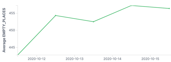
The problem is that the application only sees the DATE field, so you end up with all the values bunched into a daily aggregation. We need to be able to bring in the TIME component too in order to plot the data with any kind of granularity:

ksqlDB provides the STRINGTOTIMESTAMP function, which stores the timestamp as a native format (milliseconds since the Unix epoch). Downstream applications can consume this directly, or we can map it back to a string as needed with TIMESTAMPTOSTRING.
Here we concatenate the two fields DATE and TIME and manually specify the timezone too:
CREATE STREAM EXAMPLE_04 AS
    SELECT *,
           STRINGTOTIMESTAMP(DATE + ' ' + TIME ,
                             'yyyy-MM-dd HH:mm',
                             'Europe/London') AS TS
    FROM CARPARK_01;
Create a struct (nested field) to hold the location latitude/longitude pair
Not all heroes wear capes, and not all data structures are flat. Sometimes storing data in a nested form is useful. An example is location, in which the pair of latitude and longitude makes more sense if combined into a field called location. For example, instead of storing the following data structure:
{
  "NAME": "NCP Hall Ings",
  "LATITUDE": 53.791838,
  "LONGITUDE": -1.752201
}
we store this:
{
  "NAME": "NCP Hall Ings",
  "LOCATION": {
    "lat": 53.791838,
    "lon": -1.752201
  }
}
One good use of this is that it makes ingesting the data into Elasticsearch easier as the struct can be picked up as a geopoint type.
To create a struct, use the STRUCT() constructor:
CREATE STREAM EXAMPLE_05 AS
    SELECT *,
            STRUCT("lat" := LATITUDE,
                   "lon" := LONGITUDE) AS LOCATION
    FROM CARPARK_01;
You can also create MAP and ARRAY types in your output stream.
Create a calculated field
Finally, as well as adding static fields and nesting existing ones, we can add derived fields, such as a calculation. This is an example that works out the percentage of parking spaces that are available:
CREATE STREAM EXAMPLE_06 AS
    SELECT *,
            (CAST((CAPACITY - EMPTY_PLACES) AS DOUBLE) /
             CAST(CAPACITY AS DOUBLE)) * 100 AS PCT_FULL
    FROM CARPARK_01;
Note how the INT source fields are CAST to DOUBLE in the calculation, otherwise you don’t end up with the result you’d expect:
SELECT CAPACITY,
       EMPTY_PLACES,
       (CAST((CAPACITY - EMPTY_PLACES) AS DOUBLE) / CAST(CAPACITY AS DOUBLE)) * 100 AS PCT_FULL_DOUBLE,
       ((CAPACITY - EMPTY_PLACES) / CAPACITY) * 100 AS PCT_FULL_INT
FROM CARPARK_01 EMIT CHANGES LIMIT 5;
+-----------+--------------+--------------------+-------------+
|CAPACITY   |EMPTY_PLACES  |PCT_FULL_DOUBLE     |PCT_FULL_INT |
+-----------+--------------+--------------------+-------------+
|611        |539           |11.783960720130933  |0            |
|98         |78            |20.408163265306122  |0            |
|116        |97            |16.379310344827587  |0            |
|996        |940           |5.622489959839357   |0            |
|116        |98            |15.517241379310345  |0            |
Putting it all together
Combining all of the above techniques provides a single transformation process to run against the original source stream of data to which we applied the schema. It’s going to process every existing message in the topic (auto.offset.reset is earliest) and then every new message that arrives, writing all of this in a stream to a new topic:
SET 'auto.offset.reset' = 'earliest';

CREATE STREAM CARPARK_EVENTS
  WITH (VALUE_FORMAT='PROTOBUF',
        KAFKA_TOPIC ='carpark_events_03',
        PARTITIONS=6) AS
  SELECT *,
         STRINGTOTIMESTAMP(DATE + ' ' + TIME,
                           'yyyy-MM-dd HH:mm',
                           'Europe/London') AS TS,
         (CAST((CAPACITY - EMPTY_PLACES) AS DOUBLE) /
          CAST(CAPACITY AS DOUBLE)) * 100 AS PCT_FULL,
         STRUCT("lat" := LATITUDE,
                "lon" := LONGITUDE) AS LOCATION,
         'v2/Council/CarParkCurrent' AS SOURCE
   FROM CARPARK_SRC EMIT CHANGES;
This transforms the source CSV messages:
2020-10-06,14:41,Westgate,116,89,Spaces,53.796291,-1.759143,"https://maps.google.com/?daddr=53.796291,-1.759143"
Into messages on a target topic serialised with Protobuf:
{
  "NAME": "Westgate",
  "DATE": "2020-10-11",
  "TIME": "22:25",
  "CAPACITY": 116,
  "EMPTY_PLACES": 116,
  "STATUS": "Closed",
  "LATITUDE": 53.796291,
  "LONGITUDE": -1.759143,
  "DIRECTIONSURL": "https://maps.google.com/?daddr=53.796291,-1.759143",
  "TS": 1602451500000,
  "PCT_FULL": 0,
  "LOCATION": {
    "lat": 53.796291,
    "lon": -1.759143
  },
  "SOURCE": "v2/Council/CarParkCurrent"
}
Streaming data from Kafka in Confluent Cloud to Elasticsearch in Elastic Cloud
With the data on a Kafka topic, any application can consume it directly using the consumer API. In the above example, however, the data is used for analytics—and writing some code with the consumer API to stream the data from Kafka to a target datastore would just be ungainly. Kafka Connect exists for this reason. As part of Apache Kafka, Kafka Connect enables you to stream data from Kafka down to numerous target systems. It also works the other way, streaming data from source systems such as RDBMS or message queues into Kafka.
When self-managing Kafka, you also run the Kafka Connect worker yourself. Fortunately, in the same way that Confluent Cloud removes the worry and hassle for installing and running Kafka brokers, it does the same for Kafka Connect. By providing multiple managed connectors, Confluent Cloud makes it as easy as selecting your integration from a list, setting up the configuration, and letting Confluent Cloud do the rest for you.
I’m using Elastic Cloud for my managed Elasticsearch instance, which means that I can use the Elasticsearch Service Sink:
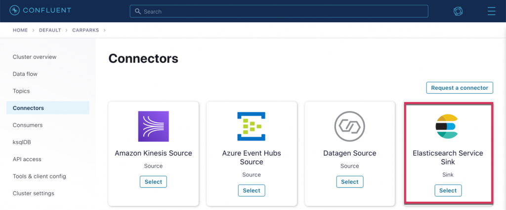
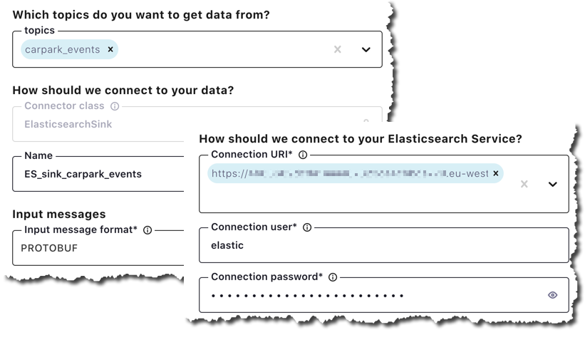
Setting the sink connector up is simple: specify the topic(s) from which you want to stream data, the target details of your Elastic Cloud endpoint, and a few other details:
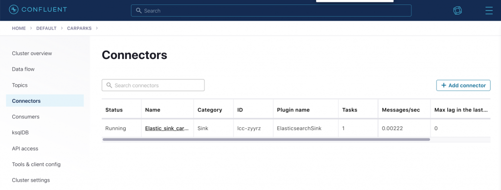
After launching the connector, you’ll see it listed as well as information such as the rate at which it’s transferring messages, current lag, and more.
In Elasticsearch, the index has been created:
 Index management within Kibana
With the data in Elasticsearch, you can analyse it to your heart’s content using Kibana, which is also provided with your Elastic Cloud deployment.
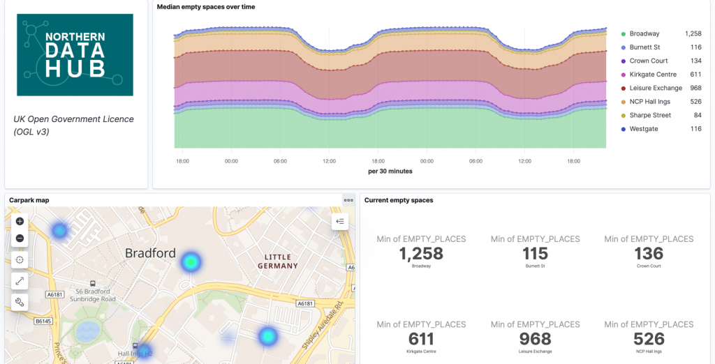 The parking dashboard in Kibana—check out the hotspot of empty spaces available in the north of the city.
Merging Kafka topics – Part 1: Past and present
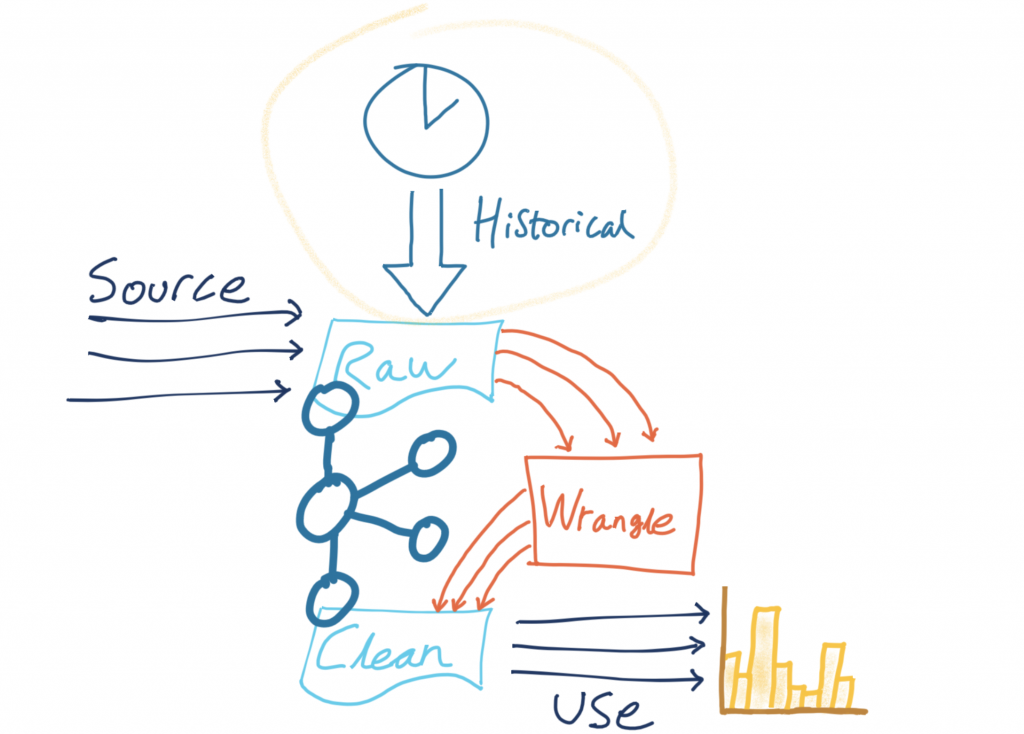
At the moment, the pipeline that we’ve built is ingesting real-time data from the source API.

There’s also an API that provides historical data. It follows mostly the same schema as the source one, so it makes sense to combine the resulting topic. Logically, it’s the same entity, just about events at different times.
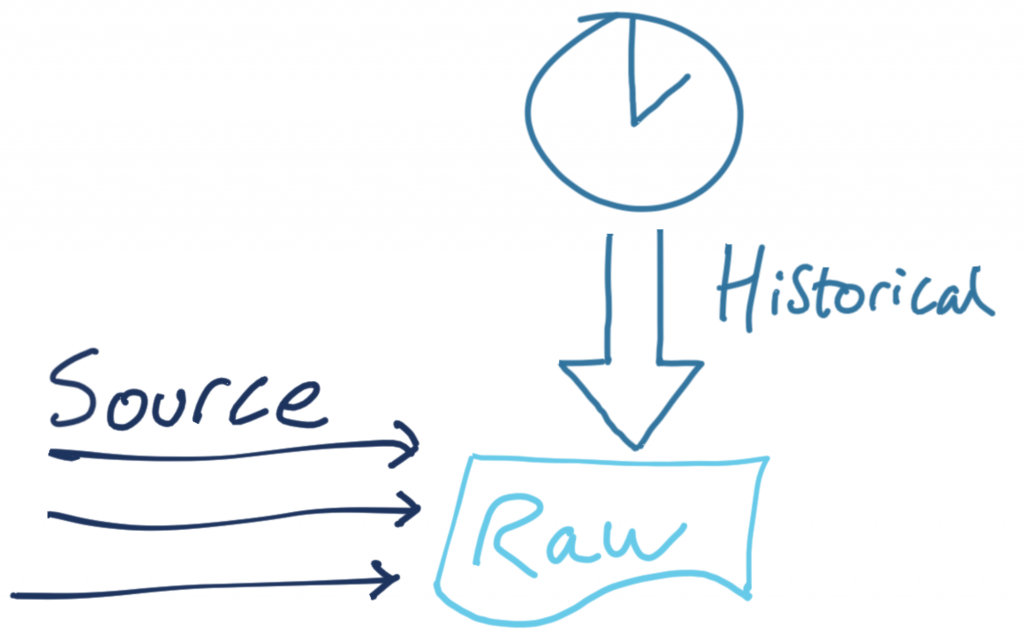
The historic data is also in CSV format:
2018-02-05,09:55,Westgate,116,80,Spaces,53.796291,-1.759143
The only difference is that it doesn’t include one of the fields (directionsURL), so we need to accommodate for that in how we handle the data.
First, we follow the same pattern as before and declare a ksqlDB stream over the data:
CREATE STREAM CARPARK_HISTORIC (date          VARCHAR ,
                                time          VARCHAR ,
                                name          VARCHAR ,
                                capacity      INT ,
                                empty_places  INT ,
                                status        VARCHAR ,
                                latitude      DOUBLE ,
                                longitude     DOUBLE )
                WITH (KAFKA_TOPIC='carparks_historic',
                VALUE_FORMAT='DELIMITED');
Now, using the INSERT INTO statement, we can apply the same set of transformations as above but writing the results to an existing ksqlDB stream (and thus an existing Kafka topic):
SET 'auto.offset.reset' = 'earliest';

INSERT INTO CARPARK_EVENTS
SELECT *,
       '' AS DIRECTIONSURL,
       STRINGTOTIMESTAMP(DATE + ' ' + TIME,
                         'yyyy-MM-dd HH:mm',
                         'Europe/London' ) AS TS,
       (CAST((CAPACITY - EMPTY_PLACES) AS DOUBLE) /
        CAST(CAPACITY AS DOUBLE)) * 100 AS PCT_FULL,
       STRUCT("lat" := LATITUDE,
              "lon" := LONGITUDE) AS LOCATION,
       'v2/Council/CarParkHistoric' AS SOURCE
  FROM CARPARK_HISTORIC
  EMIT CHANGES;
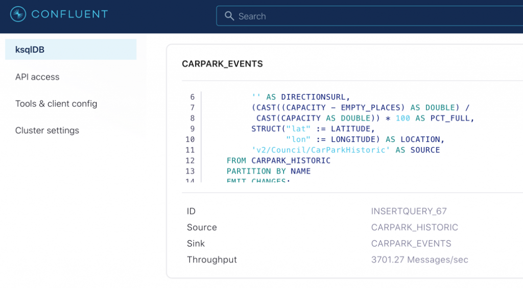
If you head over to the ksqlDB Running queries tab (or run SHOW QUERIES; from ksqlDB itself), you’ll see the INSERT is running, writing its output to the CARPARK_EVENTS stream:
Using ksqlDB’s aggregation, we can check the number of messages from each original source stream (thanks to our the addition of the lineage information above):
SELECT SOURCE,
       COUNT(*) AS EVENT_CT,
       TIMESTAMPTOSTRING(MIN(TS),'yyyy-MM-dd HH:mm:ss','Europe/London') AS EARLIEST_TS,
       TIMESTAMPTOSTRING(MAX(TS),'yyyy-MM-dd HH:mm:ss','Europe/London') AS LATEST_TS
  FROM CARPARK_EVENTS
GROUP BY SOURCE
EMIT CHANGES;

Because we’re already streaming the topic that backs this stream to Elasticsearch, the same data flows to Elasticsearch without us needing to change a thing with the connector:

Merging Kafka topics – Part 2: Round pegs into square holes
In the example above, we simply unified two pretty similar streams of data. What if we have the same logical data (car park status events) but from a completely different format?
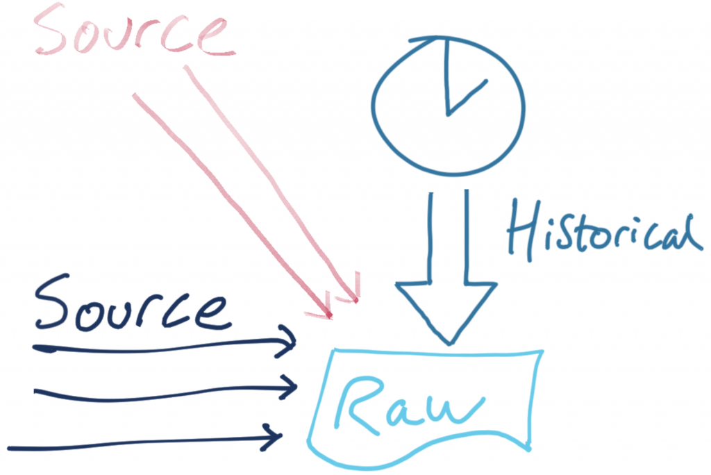
The source for this example is a JSON object, extracted from the feed provided by the Leeds City Council:
{
    "d2lm:situationRecordCreationTime": "2020-10-20T11:34:02",
    "d2lm:groupOfLocations": {
        "d2lm:locationContainedInGroup": {
            "d2lm:pointByCoordinates": {
                "d2lm:pointCoordinates": {
                    "d2lm:latitude": "53.795147075173155",
                    "d2lm:longitude": "-1.544524058364228"
                }
            }
        }
    },
    "d2lm:carParkIdentity": "Trinity Leeds:LEEDSCP0014",
    "d2lm:carParkOccupancy": "93",
    "d2lm:carParkStatus": "enoughSpacesAvailable",
    "d2lm:occupiedSpaces": "531",
    "d2lm:totalCapacity": "570"
}
First, we map the schema based on the source data:
CREATE STREAM CARPARK_LEEDS_SRC01 (
"d2lm:situationRecordCreationTime" VARCHAR,
    "d2lm:groupOfLocations" STRUCT <
        "d2lm:locationContainedInGroup" STRUCT <
            "d2lm:pointByCoordinates" STRUCT <
                "d2lm:pointCoordinates" STRUCT <
                    "d2lm:latitude" DOUBLE,
                    "d2lm:longitude" DOUBLE > > > >,
    "d2lm:carParkIdentity" VARCHAR,
    "d2lm:carParkOccupancy" DOUBLE,
    "d2lm:carParkStatus" VARCHAR,
    "d2lm:occupiedSpaces" INT,
    "d2lm:totalCapacity"  INT
    )
WITH (KAFKA_TOPIC='carparks_leeds',
      VALUE_FORMAT='JSON');
Then, we wrangle it into the same shape as our existing data:
INSERT INTO CARPARK_EVENTS
    SELECT  TIMESTAMPTOSTRING(STRINGTOTIMESTAMP("d2lm:situationRecordCreationTime",
                            'yyyy-MM-dd''T''HH:mm:ss',
                            'Europe/London'),
                            'yyyy-MM-dd')
                                    AS DATE,
            TIMESTAMPTOSTRING(STRINGTOTIMESTAMP("d2lm:situationRecordCreationTime",
                                    'yyyy-MM-dd''T''HH:mm:ss',
                                    'Europe/London'),
                                    'HH:mm')
                                    AS TIME,
            "d2lm:carParkIdentity"  AS NAME,
            "d2lm:totalCapacity"    AS CAPACITY,
            "d2lm:totalCapacity" - "d2lm:occupiedSpaces"
                                    AS EMPTY_PLACES,
            "d2lm:carParkStatus"    AS STATUS,
            "d2lm:groupOfLocations" -> "d2lm:locationContainedInGroup" -> "d2lm:pointByCoordinates" -> "d2lm:pointCoordinates" -> "d2lm:latitude"
                                    AS LATITUDE,
            "d2lm:groupOfLocations" -> "d2lm:locationContainedInGroup" -> "d2lm:pointByCoordinates" -> "d2lm:pointCoordinates" -> "d2lm:longitude"
                                    AS LONGITUDE,
            ''                      AS DIRECTIONSURL,
            STRINGTOTIMESTAMP("d2lm:situationRecordCreationTime",
                              'yyyy-MM-dd''T''HH:mm:ss',
                              'Europe/London')
                                    AS TS,
            "d2lm:carParkOccupancy" AS PCT_FULL ,
            STRUCT("lat" := "d2lm:groupOfLocations" -> "d2lm:locationContainedInGroup" -> "d2lm:pointByCoordinates" -> "d2lm:pointCoordinates" -> "d2lm:latitude",
                   "lon" := "d2lm:groupOfLocations" -> "d2lm:locationContainedInGroup" -> "d2lm:pointByCoordinates" -> "d2lm:pointCoordinates" -> "d2lm:longitude")
                                    AS LOCATION,
            'https://datamillnorth.org/dataset/live-car-park-spaces-api'
                                    AS SOURCE
            FROM  CARPARK_LEEDS_SRC01
        EMIT CHANGES;
As a result, we now have a live stream of carpark update events in a single Kafka topic but originating from multiple sources:
ksql> SELECT TIMESTAMPTOSTRING(ROWTIME,'yyyy-MM-dd HH:mm:ss','Europe/London') AS TS,
             NAME,
             CAPACITY,
             EMPTY_PLACES,
             SOURCE
        FROM CARPARK_EVENTS
        EMIT CHANGES;
+----------------------+----------------------------------+-----------+--------------+------------------------------------------------------------+
|TS                    |NAME                              |CAPACITY   |EMPTY_PLACES  | SOURCE                                                     |
+----------------------+----------------------------------+-----------+--------------+------------------------------------------------------------+
|2020-10-20 13:15:55   |Dewsbury Stn Sth:KCP13            |140        |80            | https://datamillnorth.org/dataset/live-car-park-spaces-api |
|2020-10-20 13:15:55   |Markets Multi-Storey:LEEDSCP0011  |646        |244           | https://datamillnorth.org/dataset/live-car-park-spaces-api |
|2020-10-20 13:15:55   |Trinity Leeds:LEEDSCP0014         |570        |10            | https://datamillnorth.org/dataset/live-car-park-spaces-api |
|2020-10-20 13:15:55   |The Core:LEEDSCP0002              |313        |52            | https://datamillnorth.org/dataset/live-car-park-spaces-api |
|2020-10-20 13:15:59   |Crown Court                       |142        |92            | v2/Council/CarParkCurrent                                  |
|2020-10-20 13:15:59   |Leisure Exchange                  |996        |931           | v2/Council/CarParkCurrent                                  |
|2020-10-20 13:15:59   |NCP Hall Ings                     |526        |497           | v2/Council/CarParkCurrent                                  |
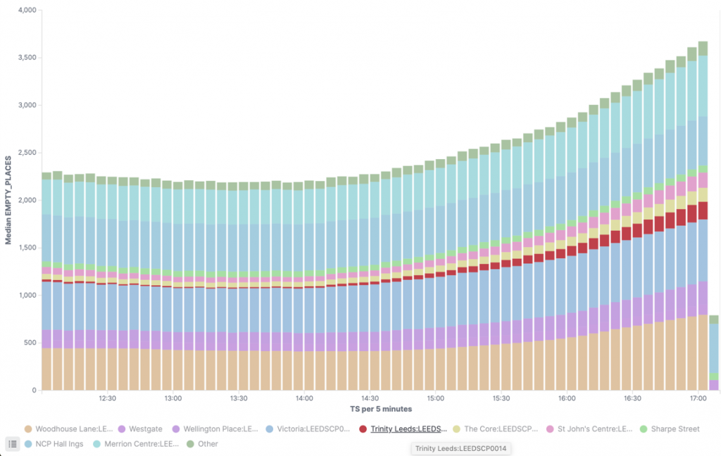 Finding parking spots in Leeds and stacking histograms in Kibana
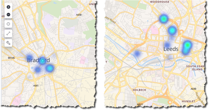 Parking heat maps in Kibana. Drive to the warmth!
Flexible pipelines
You may have noticed in the previous sections that whilst new sources of data have been added, the remainder of the pipeline (the wrangling and the consumption into Elasticsearch for analytics) remains untouched.
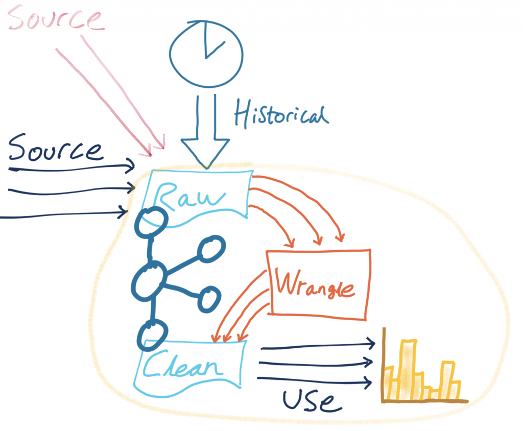
Kafka provides the benefit of creating more loosely coupled architectures that can be quickly modified and iterated upon to meet changing requirements, all whilst reducing the risk of impact to other areas.
Try it out now!
By processing streams of data in Kafka using ksqlDB we can build powerful derivations of the data for use by both applications and pipelines. There are many common patterns that are frequently required, such as applying a schema, calculating new fields, and converting data types. By applying these to a stream of data and writing it back into Kafka we make it available for others to use without introducing unnecessary dependencies.
We can also apply the necessary wrangling of data to align schemas such that multiple common streams of data can be unified into a single stream and seamlessly introduced to existing targets.
- To try this out for yourself, sign up for Confluent Cloud. You can use the promo code RMOFF200 for $200 off your bill on top of the $400 that you also get to spend within Confluent Cloud during your first 60 days. The source code for the examples in this article can be found on GitHub.
- To try out ksqlDB without the fun(?) of carpark data, check out the quickstart tutorial.
- To learn more about Elasticsearch and Kibana, get a free trial of Elastic Cloud or deploy the Elastic Stack locally.
In addition, find more examples of what you can do with a humble set of car park data in this talk: 🤖 Building a Telegram bot with Go, Apache Kafka and ksqlDB.
The data used in this example has been licensed under UK Open Government Licence (OGL v3) and is from two sources:
- Bradford car parks data. © City of Bradford Metropolitan District Council.
- Live car park spaces API, © Leeds City Council, 2020.
Avez-vous aimé cet article de blog ? Partagez-le !
Abonnez-vous au blog Confluent
Stop Treating Your LLM Like a Database
GenAI thrives on real-time contextual data: In a modern system, LLMs should be designed to engage, synthesize, and contribute, rather than to simply serve as queryable data stores.
Generative AI Meets Data Streaming (Part III) – Scaling AI in Real Time: Data Streaming and Event-Driven Architecture
In this final part of the blog series, we bring it all together by exploring data streaming platforms (DSPs), event-driven architecture (EDA), and real-time data processing to scale AI-powered solutions across your organization.

