[Virtuelles Event] GenAI Streamposium: Lerne, Echtzeit-GenAI-Apps zu entwickeln und zu skalieren | Jetzt registrieren
Getting Started Analyzing Twitter Data in Apache Kafka through KSQL
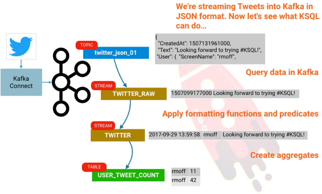
KSQL is the streaming SQL engine for Apache Kafka®. It lets you do sophisticated stream processing on Kafka topics, easily, using a simple and interactive SQL interface. In this short article we’ll see how easy it is to get up and running with a sandbox for exploring it, using everyone’s favorite demo streaming data source: Twitter. We’ll go from ingesting the raw stream of tweets, through to filtering it with predicates in KSQL, to building aggregates such as counting the number of tweets per user per hour.

First up, go grab a copy of Confluent Platform. I’m using the RPM but you can use tar, zip, etc. if you want to. Start the Confluent stack up:
$ confluent start
(Here’s a quick tutorial on the confluent CLI if you’re interested!)
We’ll use Kafka Connect to pull the data from Twitter. The Twitter Connector can be found GitHub. To install it, simply do the following:
# Clone the git repo
cd /home/rmoff
git clone https://github.com/jcustenborder/kafka-connect-twitter.git
# Compile the code
cd kafka-connect-twitter
mvn clean package
Once successfully built, unpack the resulting archive in order for Connect to use it:
cd target
tar -xvf kafka-connect-twitter-0.2-SNAPSHOT.tar.gz
To get Kafka Connect to pick up the connector that we’ve built, you’ll have to modify the configuration file. Since we’re using the Confluent CLI, the configuration file is actually etc/schema-registry/connect-avro-distributed.properties, so go modify that and add to it:
plugin.path=share/java,/home/rmoff/kafka-connect-twitter/
Restart Kafka Connect:
confluent stop connect
confluent start connect
Once you’ve installed the plugin, you can easily configure it. You can use the Kafka Connect REST API directly, or create your configuration file, which is what I’ll do here. You’ll need to head over to Twitter to grab your API keys first.
Assuming you’ve written this to /home/rmoff/twitter-source.json, you can now run:
$ confluent load twitter_source -d /home/rmoff/twitter-source.json
And then tweets from everyone’s favourite internet meme star start [rick]-rolling in…
Now let’s fire up KSQL! KSQL is included with Confluent Platform 4.1 onwards. Assuming you’ve used Confluent CLI to start things up, this will also have started the KSQL server, and you can simply run:
ksql
Using KSQL, we can take our data that’s held in Kafka topics and query it. First, we need to tell KSQL what the schema of the data in the topic is. A twitter message is actually a pretty huge JSON object, but for brevity let’s just pick a couple of columns to start with:
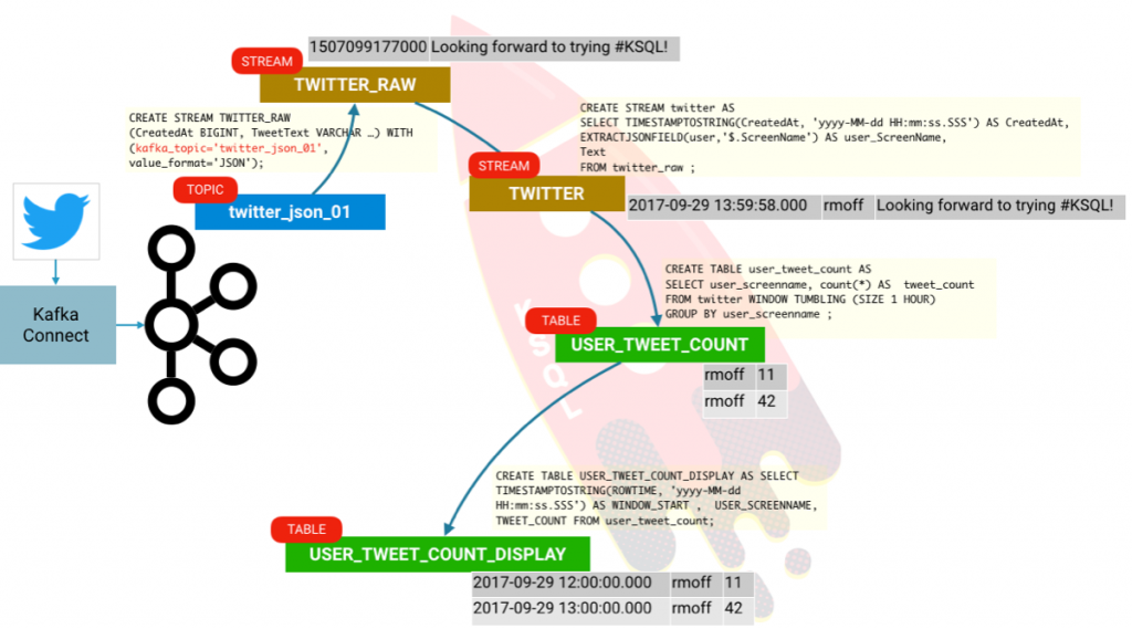
ksql> CREATE STREAM twitter_raw (CreatedAt BIGINT, Id BIGINT, Text VARCHAR) WITH (KAFKA_TOPIC='twitter_json_01', VALUE_FORMAT='JSON');
Message
----------------
Stream created
With the schema defined, we can query the stream. To get KSQL to show data from the start of the topic (rather than the current point in time, which is the default), run:
ksql> SET 'auto.offset.reset' = 'earliest';
Successfully changed local property 'auto.offset.reset' from 'null' to 'earliest'
And now let’s see the data. We’ll select just one row using the LIMIT clause:
Now let’s redefine the stream with all the contents of the tweet payload now defined and available to us:
Now we can manipulate and examine our data more closely, using normal SQL queries:
Note that there’s no LIMIT clause, so you’ll see on screen the results of the continuous query. Unlike a query on a relational table that returns a definite number of results, a continuous query is running on unbounded streaming data, so it always has the potential to return more records. Hit Ctrl-C to cancel and return to the KSQL prompt. In the above query we’re doing a few things:
- TIMESTAMPTOSTRING to convert the timestamp from epoch to a human-readable format
- EXTRACTJSONFIELD to show one of the nested user fields from the source, which looks like:
- Applying predicates to what’s shown, using pattern matching against the hashtag, forced to lower case with LCASE.
For a list of supported functions, see the KSQL documentation.
We can create a derived stream from this data:
and query the derived stream:
Before we finish, let’s see how to do some aggregation.
You’ll probably get a screenful of results; this is because KSQL is actually emitting the aggregation values for the given hourly window each time it updates. Since we’ve set KSQL to read all messages on the topic (SET 'auto.offset.reset' = 'earliest';) it’s reading all of these messages at once and calculating the aggregation updates as it goes. There’s actually a subtlety in what’s going on here that’s worth digging into. Our inbound stream of tweets is just that—a stream. But now that we are creating aggregates, we have actually created a table. A table is a snapshot of a given key’s values at a given point in time. KSQL aggregates data based on the event time of the message, and handles late arriving data by simply restating that relevant window if it updates. Confused? We hope not, but let’s see if we can illustrate this with an example. We’ll declare our aggregate as an actual table:
Looking at the columns in the table, there are two implicit ones in addition to those we asked for:
ksql> DESCRIBE user_tweet_count;
Field | Type
-----------------------------------
ROWTIME | BIGINT
ROWKEY | VARCHAR(STRING)
USER_SCREENNAME | VARCHAR(STRING)
TWEET_COUNT | BIGINT
ksql>
Let’s see what’s in these:
The ROWTIME is the window start time, the ROWKEY is a composite of the GROUP BY (USER_SCREENNAME) plus the window. So we can tidy this up a bit by creating an additional derived table:
Now it’s easy to query and see the data that we’re interested in:
Conclusion
So there we have it! We’re taking data from Kafka, and easily exploring it using KSQL. Not only can we explore and transform the data, we can use KSQL to easily build stream processing from streams and tables.

If you’re interested in more, check out:
- Our KSQL webinar and Kafka Summit keynote
- The clickstream demo that’s detailed in the KSQL Documentation
- A presentation that I did showing how KSQL can underpin a streaming ETL based platform
- ksqlDB, the successor to KSQL, and see the latest syntax
Ist dieser Blog-Beitrag interessant? Jetzt teilen
Confluent-Blog abonnieren
Stop Treating Your LLM Like a Database
GenAI thrives on real-time contextual data: In a modern system, LLMs should be designed to engage, synthesize, and contribute, rather than to simply serve as queryable data stores.
Generative AI Meets Data Streaming (Part III) – Scaling AI in Real Time: Data Streaming and Event-Driven Architecture
In this final part of the blog series, we bring it all together by exploring data streaming platforms (DSPs), event-driven architecture (EDA), and real-time data processing to scale AI-powered solutions across your organization.

