[Webinar] AI-Powered Innovation with Confluent & Microsoft Azure | Register Now
Using Graph Processing for Kafka Streams Visualizations
We know that Apache Kafka® is great when you’re dealing with streams, allowing you to conveniently look at streams as tables. Stream processing engines like ksqlDB furthermore give you the ability to manipulate all of this fluently.
But what about when the relationships between items dominate your application? For example, in a social network, understanding the network means we need to look at the friend relationships between people. In a financial fraud application, we need to understand flows of money between accounts. In an identity/access management application, it’s the relationships between roles and their privileges that matters most.
If you’ve found yourself needing to write very large JOIN statements or dealing with long paths through your data, then you are probably facing a graph problem. Looking at your data as a graph pays off tremendously when the connections between individual data items are as valuable as the items themselves. Many domains, such as social relationships, company ownership structures, and even how web pages link to one another on the web are very naturally a graph.
Kafka already allows you to look at data as streams or tables; graphs are a third option, a more natural representation with a lot of grounding in theory for some use cases. So we can improve a portion of just about any event streaming application by adding graph abilities to it. Just as we use streams and tables for the portions that best benefit from those ways of thinking about our data, we can use graph abilities where they make sense to more easily approach our use case.
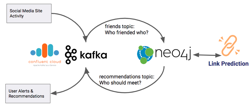
If you’re looking for the basics on how you can turn streams into graphs with Neo4j and the Neo4j-Streams plugin, you’ve come to the right place. We will cover how you can use them to enrich and visualize your data, add value to it with powerful graph algorithms, and then send the result right back to Kafka. You can use this as an example of how to add graph abilities to any event streaming application.
We will also be using Confluent Cloud, which provides a fully managed event streaming service based on Apache Kafka. I like Confluent Cloud because it lets me focus on getting the value of Kafka without the management and maintenance overhead of extra infrastructure. I get to spin up Kafka in a few minutes, scaling is taken care of for me, and there’s never any patching or restarting to worry about. The approach we’ll use works with any Kafka run though.
All of the code and setup discussed in this blog post can be found in this GitHub repository, so you can try it yourself!
A stream of friend relationships
Suppose we’re operating a social network site, and we have a stream of simple records that let us know who is friending who on the platform. We’ll strip down the data example to something very simple so we can focus on the concepts:
{"initiated": "Cory", "accepted": "Levi", "friends": true, "date": "2019-08-08T16:13:11.774754"}
{"initiated": "Shana", "accepted": "Avi", "friends": true, "date": "2019-08-08T16:13:11.996435"}
{"initiated": "Tsika", "accepted": "Maura", "friends": true, "date": "2019-08-08T16:13:12.217716"}
Here, we have three sample records moving over the “friends” topic in Kafka. “Corey” initiated a friend request to “Levi”, which was accepted on Aug. 8, and so on.
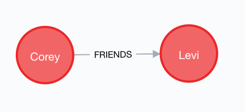
A stream of these records is going to create a natural graph of individuals and their friendships. Each time we add a friend record, we simply create the person if they don’t already exist and link them up. Repeating this over and over with simple pairwise relationships, like what you see above, results in what you see below.
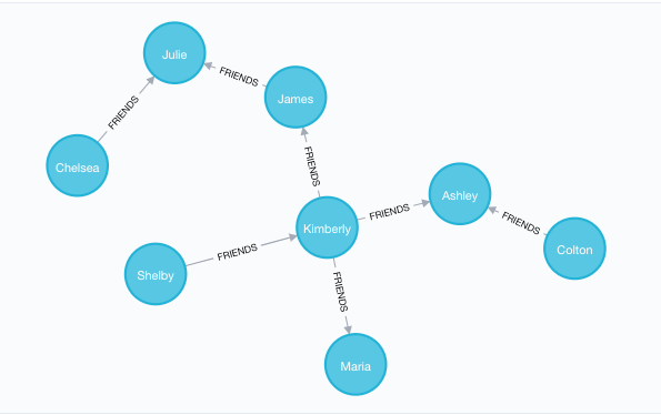
Suppose we had a few million of these “friendships,” and we wanted to know who was a friend of a friend of David’s. That would take at least a three-way table join. If we wanted to know how many people were between four and six degrees of separation away from David…well, you can try to write that in SQL if you like—good luck!
It’s time to call upon the graph hero for this event streaming application. Here we go!
Step 1: Graph the network with Neo4j
We’ll be using Neo4j, which is a native graph database. Instead of storing tables and columns, Neo4j represents all data as a graph, meaning that the data is a set of nodes with labels and relationships. Nodes are like our data entities (in this example, we use Person). Relationships act like verbs in your graph. For example, Cory FRIENDED Levi. This approach to structuring data is called the property graph model.
To query a property graph, we’ll be using the Cypher language, which is a declarative query language similar to SQL, but for graphs. With Cypher, you can describe patterns in graphs as a sort of ascii art; for example in this query:
MATCH (p1:Person)-[:FRIENDS]->(p2:Person)
RETURN *;
Neo4j would find sets of two Person nodes that are related by a FRIENDS relationship, and return everything that it found. Nodes are always enclosed in round brackets, with relationships in square brackets.
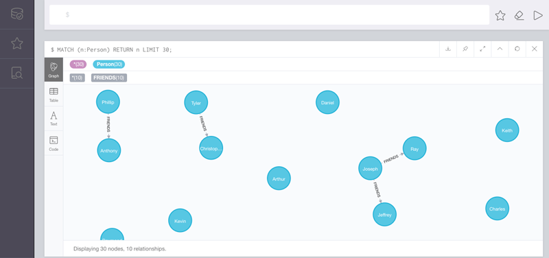
When you start a Neo4j instance, it comes with Neo4j Browser, an application that runs on port 7474 of the host, and provides an interactive Cypher query shell, along with visualization of the results. In this blog post when you see pictures of graphs or Cypher queries, we are using Neo4j Browser to enter those queries and see the result, as seen below.
In the code repo that accompanies this post, the setup has mostly been done for you in the form of a Docker Compose file. This will work right out of the box if you’re familiar with Docker—just clone the repo, and execute docker-compose up to get running. These instructions generally follow what you’ll find in the documentation quick start instructions. Neo4j Streams lets Neo4j act as either a source or sink of data from Kafka. Extensive documentation is available, but let’s just skip to the good parts and make this work.
Note: users also have the option of using the Kafka Connect Neo4j Sink instead of the plugin we’re using in this article. We use the plugin to keep the deployed stack as simple to understand as possible, and also because it supports producing data back to Kafka in addition to sinking data.
The code repo we are using for this example includes:
- Docker Compose information that lets us create the necessary Neo4j infrastructure
- Configuration that attaches it to a Confluent Cloud instance
- A submodule which allows us to generate synthetic JSON objects and send them to Kafka (called “fakestream”)
- Scripts that allow us to prime our use case with some sample data
Configuring Neo4j to interact with Kafka
Open up the docker-compose.yml file, and you will see the following:
     NEO4J_kafka_group_id: p2
     NEO4J_streams_sink_topic_cypher_friends: "
       MERGE (p1:Person { name: event.initiated })
       MERGE (p2:Person { name: event.accepted })
       CREATE (p1)-[:FRIENDS { when: event.date }]->(p2)
     "
     NEO4J_streams_sink_enabled: "true"
     NEO4J_streams_procedures_enabled: "true"
     NEO4J_streams_source_enabled: "false"
     NEO4J_kafka_ssl_endpoint_identification_algorithm: https
     NEO4J_kafka_sasl_mechanism: PLAIN
     NEO4J_kafka_request_timeout_ms: 20000
     NEO4J_kafka_bootstrap_servers: ${KAFKA_BOOTSTRAP_SERVERS}
     NEO4J_kafka_retry_backoff_ms: 500
     NEO4J_kafka_sasl_jaas_config: org.apache.kafka.common.security.plain.PlainLoginModule required username="${CONFLUENT_API_KEY}" password="${CONFLUENT_API_SECRET}";
     NEO4J_kafka_security_protocol: SASL_SSL
This configuration is doing several things worth breaking down. We’re enabling the plugin to work as both a source and a sink. In the NEO4J_streams_sink_topic_cypher_friends item, we’re writing a Cypher query. In this query, we’re MERGE-ing two Person nodes. The plugin gives us a variable named event, which we can use to pull out the properties we need. When we MERGE nodes, it creates them only if they do not already exist. Finally, it creates a relationship between the two nodes (p1) and (p2).
This sink configuration is how we’ll turn a stream of records from Kafka into an ever-growing and changing graph. The rest of the configuration handles our connection to a Confluent Cloud instance, where all of our event streaming will be managed for us. If you’re trying this out for yourself, make sure to replace KAFKA_BOOTSTRAP_SERVERS, API_SECRET, and API_KEY with the values that Confluent Cloud gives you when you generate an API access key.
After starting Neo4j and allowing some of our records to be consumed from the Kafka topic, we gradually build a bigger and bigger graph that looks like this, when viewed in Neo4j Browser, which will be running on http://localhost:7474/ and can be accessed by the username and password specified in the docker-compose.yml file (neo4j/admin):
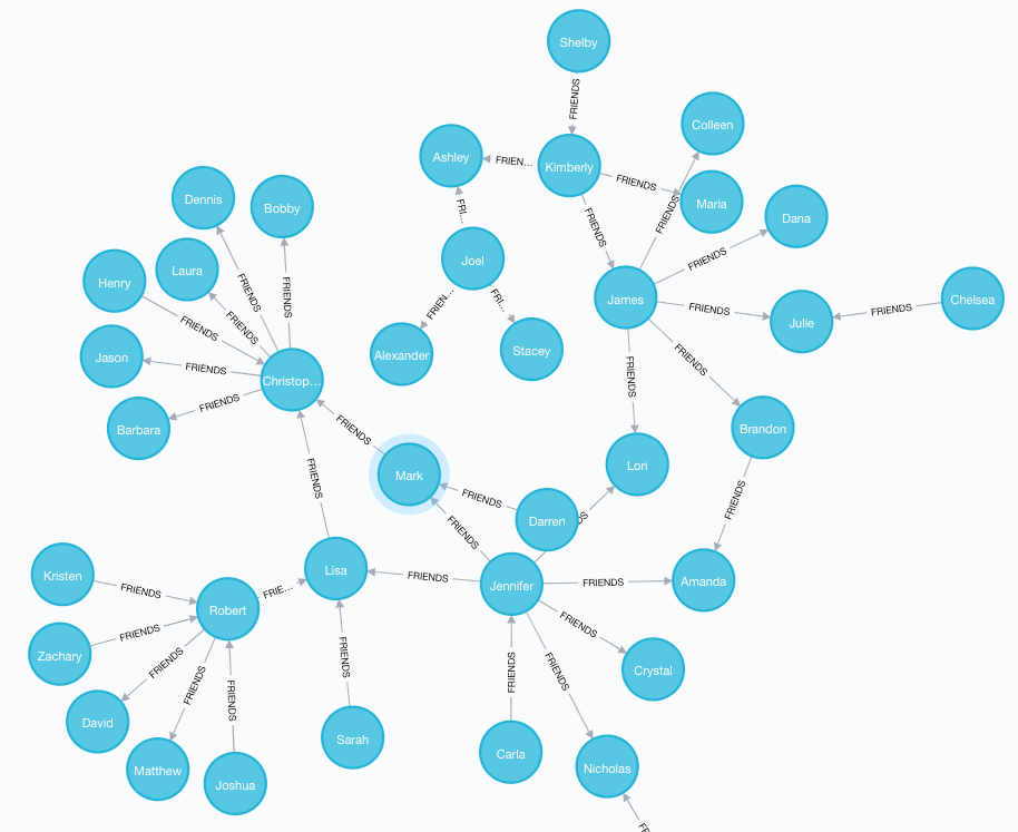
As with most social networks, there are some heavily connected people in this graph who know a lot of people, and others around the periphery with fewer friends in the network. By making this data a graph and visualizing it, we can immediately see patterns of relationships that would have been invisible in a list of records.
Step 2: Using graph algorithms to recommend potential friends
The Neo4j Graph Algorithms package that comes with Neo4j allows us to do some really interesting things with our graph. To grow our social network site, we want to encourage users to connect by suggesting potential friends. But how do we produce the most relevant results? We need a way to generate a recommendation and inject it back into a different Kafka topic so that we can drive things like emails to our users and more recommendations on the site.
Link prediction algorithms
In graph algorithms, we have a family of approaches called link prediction algorithms. They help determine the closeness of two nodes and how likely those nodes will connect to one another in the future. Using our social network example, these might be your real life friends who you already know but haven’t yet connected with. Those would make great friend recommendations!
Common Neighbors algorithm
Specifically, we’ll use an approach called the Common Neighbors algorithm. Two strangers who have a lot of friends in common are good targets to introduce to one another.
In Cypher, we’ll simply run the algorithm like so, which we can do in Neo4j Browser:
MATCH (p1:Person)-[:FRIENDS*2]-(p2:Person)
WHERE NOT (p1)-[:FRIENDS]-(p2) AND
id(p1) < id(p2)
WITH distinct(p1), p2
RETURN p1.name, p2.name, algo.linkprediction.commonNeighbors(p1, p2, {}) as score
ORDER BY score DESC;
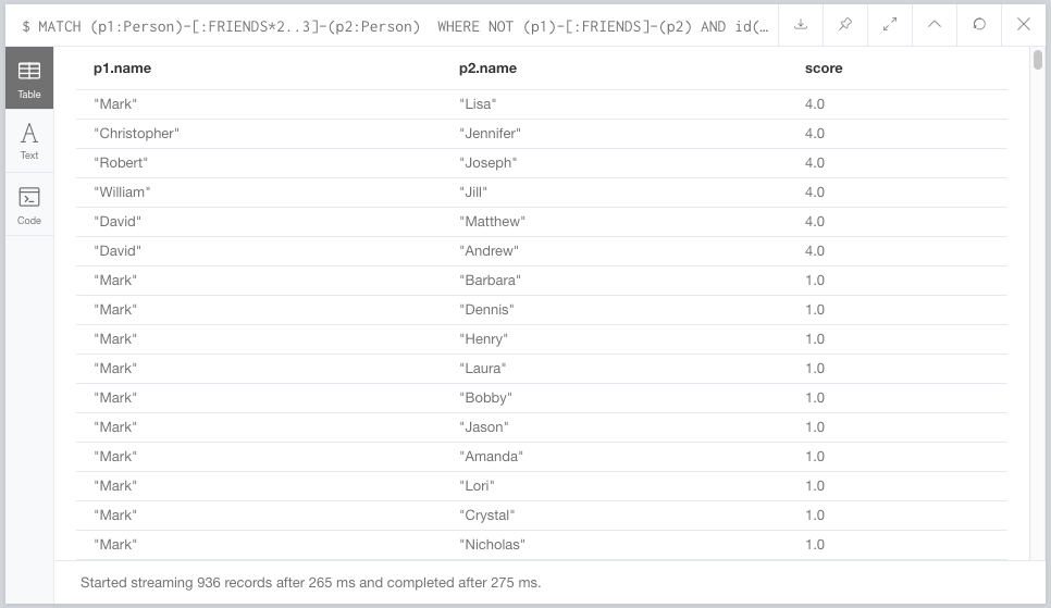
The first line finds all pairs of people who are separated by two degrees (by some path) but who are also not directly connected to one another. (We don’t want to suggest that two people friend one another when they’re already friends!)
We then call algo.linkprediction.commonNeighbors on those two nodes, return that as a score, and get a list of people and their common neighbor scores, again shown in Neo4j Browser.
Step 3: Publishing back to Kafka
OK, so far, so good. We know how to determine how many common neighbors people have, which is a good way of identifying who might friend who. But we haven’t gotten that data back into Kafka yet. Let’s look at two quick options we might consider.
Publishing ad hoc
By using the streams.publish Cypher function, we can always publish the results of any Cypher query back to Kafka. This is a key part of tying graphs and streams together easily. Anything done in Cypher can be piped back to a topic with little effort, by executing this in Neo4j Browser.
MATCH (p1:Person)-[:FRIENDS*2..3]-(p2:Person)
WHERE NOT (p1)-[:FRIENDS]-(p2) AND
id(p1) < id(p2) WITH distinct(p1), p2, algo.linkprediction.commonNeighbors(p1, p2, {}) as score WHERE score >= 2
CALL streams.publish('recommendations', { a: p1.name, b: p2.name, score: score }) RETURN null;
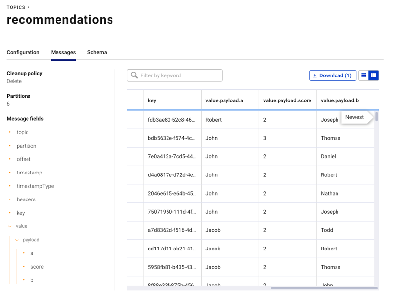
This is the same query we ran previously The only difference is that at the bottom, we limit the results to a score of two or higher and add the streams.publish call, sending it a tiny payload consisting of a, b, and score.
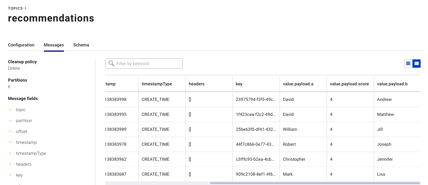
Meanwhile, in Confluent Cloud, our records arrive pretty much as you’d expect.
Publishing nodes and edges as they’re created
The weakness of the last approach is that it requires manual notification to Kafka, either scheduled or based on some type of a trigger mechanism. Sometimes though, we might want to have a separate microservice that generates recommendations. It might, for example, use the Common Neighbors approach, but also other approaches as well to make more nuanced and higher quality recommendations. A great way to decouple these concerns is to just have your recommendation engine focus on making recommendations and not worry about the Kafka bits.
As with other databases, you can also just use Neo4j as a source of data. So if your recommendation service can put new nodes into the graph, the plugin can get them to Kafka as needed. This can be done by adding a little bit of configuration to your neo4j.conf:
streams.source.enabled=true
streams.source.topic.nodes.recommendations=Recommendation{*}
The streams.source.topic.nodes.recommendations item says that we’re going to take all of the Recommendation nodes in our graph and publish them to the recommendations Kafka topic. The {*} bit says we want to publish all properties of the recommendation; you can read more about those patterns in the documentation.
To show you how that works, we’ll adjust our recommendations code one more time. Instead of publishing to Kafka, we’ll just create a recommendation node. The underlying database handles the rest.
MATCH (p1:Person)-[:FRIENDS*2..3]-(p2:Person)
WHERE NOT (p1)-[:FRIENDS]-(p2) AND
id(p1) < id(p2) WITH distinct(p1), p2, algo.linkprediction.commonNeighbors(p1, p2, {}) as score WHERE score >= 2
MERGE (r:Recommendation {
   a: p1.name,
   b: p2.name,
   score: score
})
MERGE (p1)<-[:SHOULD_FRIEND]-(r)-[:SHOULD_FRIEND]->(p2)
RETURN count(r);
Once it is run, below is a picture of the resulting recommendation graph showing how people in the social network are connected by scores. For instance, “Mark” in the center and “Matthew” at the bottom seem like they have multiple different paths that would lead them to recommend they connect!
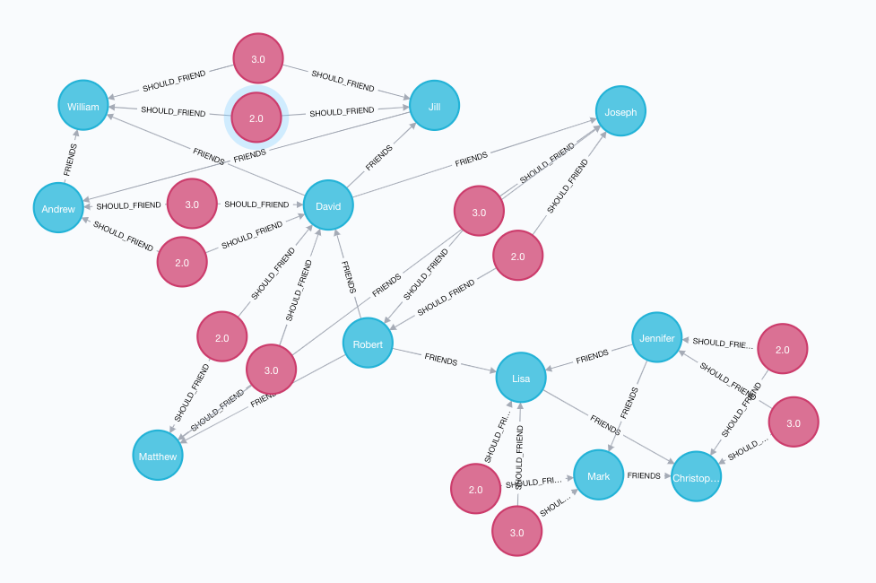
In a production scenario, a microservice would likely be responsible for generating these “recommendations,” tracking recommendations over time as data in Neo4j and letting the data publishing to Kafka take care of the rest.
Meanwhile, in Kafka, the data shows up as we expect but with some extra metadata published by the producer.
Summary
Through the simple example of a social media network and adding friends, you can take any data, turn it into a graph, leverage graph processing, and pipe the result back to Kafka. The sky’s the limit!
Whether you’re detecting Russian manipulation of elections on Twitter, looking into bank and financial fraud scenarios, pulling related transactions out of the Bitcoin blockchain, or trying to feed the world by improving crop yields, graphs are pretty much everywhere, just like streams.
When you zoom out from your architecture, this effectively allows you to add graph superpowers to just about any event streaming application. The architecture diagram in the beginning of this post shows how the process of data moving into Neo4j and back out of it again can be abstracted to just another step in a processing pipeline, enabling you to add graph analytics as necessary. If Kafka is persisting your log of messages over time, just like with any other event streaming application, you can reconstitute datasets when needed.
For anyone interested in learning more, you can check out my session from Kafka Summit San Francisco titled Extending the Stream/Table Duality into a Trinity, with Graphs, where I discuss this in more detail.
Happy stream → graph → stream hacking!
Ist dieser Blog-Beitrag interessant? Jetzt teilen
Confluent-Blog abonnieren
Stop Treating Your LLM Like a Database
GenAI thrives on real-time contextual data: In a modern system, LLMs should be designed to engage, synthesize, and contribute, rather than to simply serve as queryable data stores.
Generative AI Meets Data Streaming (Part III) – Scaling AI in Real Time: Data Streaming and Event-Driven Architecture
In this final part of the blog series, we bring it all together by exploring data streaming platforms (DSPs), event-driven architecture (EDA), and real-time data processing to scale AI-powered solutions across your organization.

