Data Enrichment in ksqlDB Using UDTFs

This blog post applies to ksqlDB version 0.8.1 and later.

Keeping a datacenter up and running is no walk in the park. It’s a job that involves mind-boggling amounts of electrical power, countless network switches, and elaborate cooling solutions. All of this needs to be monitored on a constant basis to ensure that the infrastructure is running smoothly: Are the UPS’s running on input power or battery power? Are the cooling units in tip-top shape? If there has been a power outage, have the generators started properly? What’s the bandwidth usage for each of our servers? To whom do these servers belong? What’s the power consumption for each tenant in the datacenter?

Such monitoring could be done by placing a colleague in front of a bunch of control panels and having them stare at those until a light goes from green to red, but that’s not fun for anyone, starting with the person in charge of staring at the control panels. Machines should do the boring repetitive work, while humans solve problems.

Automated monitoring is what I’ve been working on, and the likes of Logstash, Apache Kafka^®, and Elasticsearch, have been a godsend, making this not only possible but also easy and powerful. We’ve got eyes on our infrastructure, and if anything happens, notifications are immediately sent to the right people. We’ve got detailed statistics for multiple data points so that we can identify issues before they happen. But what if we wish to both monitor infrastructure and combine this monitoring with other data sources from elsewhere?

Take power consumption, for example. In one place, we have readings taken from breaker panels inside a server room. In another place, we have tenants interested in knowing their power consumption so that they remain beneath the threshold of the power commitment they signed up for. Could we export both lists into spreadsheets and have someone put them together for every reporting run? Absolutely. Does anyone want to do this? Not by a long shot. This is boring and repetitive work, so let’s give it to a machine.

This is where ksqlDB can lend a hand. In this example, we are going to create a user-defined table function (UDTF) that takes in a structure as a parameter and outputs a list of structures.

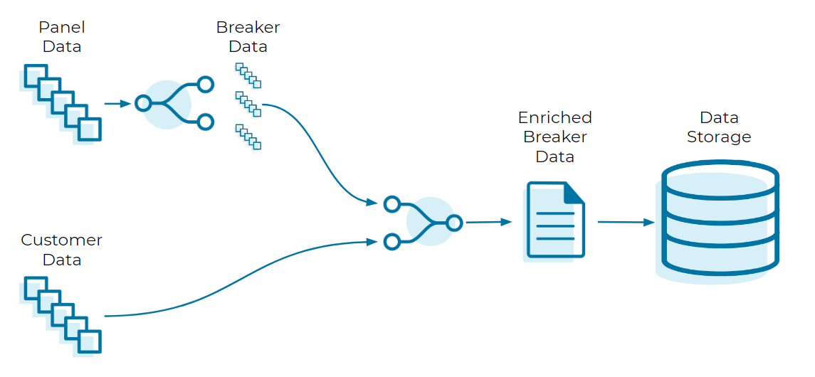
One of the biggest strengths of ksqlDB is its ability to modify and enrich data before it is sent for storage. Instead of filling a production database with data that exists in a transition phase, we submit only the final and complete version of that data, while all of the processing happens upstream. This makes for both a more natural and a more efficient way to get the data into a format that’s usable by its intended recipients. Basically, we are seeking to go from this…

To this:

While ksqlDB comes with several built-in functions, it can do so much more thanks to the power of user-defined functions (UDFs). UDFs allow us to expand ksqlDB’s functionality with anything we desire, tailored to the intended use case.

Let’s come back to our data consumption example, and express it in terms of the following scenario:

Within a building, a smart electrical panel supplies power to three tenants. We wish to monitor this panel for multiple reasons:

• Ensuring that power consumption is within prescribed safe limits
• Giving our customers visibility into their power usage statistics and history
• Using the power usage statistics to better predict peak usage times and ensure that we have the necessary infrastructure to support our customers’ usage

Let’s take a closer look at what we’re dealing with under the hood to get a better idea of our starting conditions.

The panel is located in room 01 of the first floor (hence its name) and delivers its data at regular intervals as flat JSON. An example of one reading is below:

{
    "breaker_1": 1.45,
    "breaker_2": 0.83,
    "breaker_3": 2.10,
    "system_name": "F01R01",
    "panel_number": "1",
    "@timestamp": "2020-05-19T15:53:33.899Z" 
}

Our customer information has already been processed into a proper format, in preparation for it to be linked with breaker data. An example of one customer record is below:

{
    "customer_name": "Wile Coyote, a subsidiary of Acme Inc.",
    "customer_number": 5732,
    "panel_name": "F01R01",
    "panel_number": "1",
    "breaker_number": "2"
}

Both data sources have already been pulled into a Kafka topic for each: panel_entries and customer_entries, respectively.

We face two challenges here. First, the breaker panel itself is not aware of which breaker is being used by whom. Second, we want to deliver usage statistics to customers while maintaining proper data privacy: If we were to simply hand off readings of the entire panel, a customer would see the usage of their neighbors.

In the case of the customer_entries topic, each entry has been given a key to uniquely identify it, and the key is composed of the panel name, panel number, and breaker number put together, like so: F01R01_1_2. Having a key is crucial to linking customer data with panel breaker data further down the line. No key, no data enrichment.

Our task is to connect these pieces together. This is done in three steps:

1. Create the necessary data streams/tables in ksqlDB
2. Separate the panel entries into one entry per breaker reading
3. Merge each breaker reading entry with a customer entry to enrich its data

Step 1: ksqlDB architecture

Let’s start by laying the foundations.

For the customer entries, we are interested only in the latest and greatest. Therefore, a table is the appropriate choice here:

CREATE TABLE customer_entries_table (
    customer_id VARCHAR PRIMARY KEY,
    customer_name VARCHAR,
    customer_number INT,
    panel_name VARCHAR,
    panel_number VARCHAR,
    breaker_number VARCHAR
) WITH (kafka_topic='customer_entries', value_format='json');

Next, let’s stream the panel entries:

CREATE STREAM panel_entries_stream (
    breaker_1 DOUBLE,
    breaker_2 DOUBLE,
    breaker_3 DOUBLE,
    system_name VARCHAR,
    panel_number VARCHAR
) WITH (kafka_topic='panel_entries', value_format='json');

In order to prepare the data for the UDTF, we must put it in an appropriate structure format. Thus, we must perform one additional step—converting the entry’s contents into a struct:

CREATE STREAM panel_struct AS SELECT
    STRUCT(
        "BREAKER_1" := breaker_1,
        "BREAKER_2" := breaker_2,
        "BREAKER_3" := breaker_3,
        "SYSTEM_NAME" := system_name,
        "PANEL_NUMBER" := panel_number
    ) AS panel_reading
FROM PANEL_ENTRIES_STREAM EMIT CHANGES;

This creates a new Kafka topic called panel_struct. If we examine the same entry from before, it takes a slightly different form in this topic:

{
    "PANEL_READING": {
        "BREAKER_1": 1.45,
        "BREAKER_2": 0.83,
        "BREAKER_3": 2.10,
        "SYSTEM_NAME": "F01R01"
        "PANEL_NUMBER": "1"
    }
}

Doing this allows us to supply the entire panel_reading structure as one parameter, instead of taking each field separately.

Although this does not take away the need to supply a rigid format for our UDTF, it does move that format into a spot that’s easier to maintain, update, and spawn into alternate versions in the future.

Note: We do not necessarily need to convert the entire entry into a struct, and in real-world situations, we’ll want to limit our scope a little so that the struct’s definition does not become too crowded. In our example here, however, all the fields are of interest, so we’ll put them all in. The idea is that after we have performed the split, we can still recognize where each breaker entry is coming from.

Step 2: Separate panel entries

Write the JAR file

This is where the UDTF comes in. For this, we’ll need a Java development environment of some sort and a way to build our code into a .jar file. For the sake of clarity, we will not get into the specifics of the environment or the architecture build; we will only focus on the code to write.

We need one class with the proper annotations to make it detectable by ksqlDB and recognizable as a UDTF:

import io.confluent.ksql.function.udf.UdfParameter;
import io.confluent.ksql.function.udtf.Udtf;
import io.confluent.ksql.function.udtf.UdtfDescription;
import org.apache.kafka.connect.data.Schema;
import org.apache.kafka.connect.data.SchemaBuilder;
import org.apache.kafka.connect.data.Struct;

import java.util.ArrayList;
import java.util.List;

@UdtfDescription(name="split_panel", description="Function to split a panel entry into breaker entries.")
public class SplitPanel {

   public static final String INPUT_STRUCT_DESCRIPTOR = "STRUCT<" + "BREAKER_1 DOUBLE," + "BREAKER_2 DOUBLE," + "BREAKER_3 DOUBLE," + "SYSTEM_NAME STRING," + "PANEL_NUMBER STRING" + ">";

   public static final String OUTPUT_STRUCT_DESCRIPTOR = "STRUCT<" + "READING DOUBLE," + "POSITION STRING," + "SYSTEM_NAME STRING," + "PANEL_NUMBER STRING" + ">";

   public static final Schema OUTPUT_SCHEMA = SchemaBuilder.struct().optional()
           .field("READING", Schema.OPTIONAL_FLOAT64_SCHEMA)
           .field("POSITION", Schema.OPTIONAL_STRING_SCHEMA)
           .field("SYSTEM_NAME", Schema.OPTIONAL_STRING_SCHEMA)
           .field("PANEL_NUMBER", Schema.OPTIONAL_STRING_SCHEMA)
           .build();

   @Udtf(description = "Splits a panel entry into multiple breaker sub-entries.", schema = OUTPUT_STRUCT_DESCRIPTOR)
   public List<Struct> split_panel(@UdfParameter(schema = INPUT_STRUCT_DESCRIPTOR) final Struct panelEntry) {

       List<Struct> breakerEntries = new ArrayList<>();

       for(int i=1; i <= 3; i++) {
           breakerEntries.add(new Struct(OUTPUT_SCHEMA)
                   .put("READING", panelEntry.get("BREAKER_" + i))
                   .put("POSITION", String.valueOf(i))
                   .put("SYSTEM_NAME", panelEntry.get("SYSTEM_NAME"))
                   .put("PANEL_NUMBER", panelEntry.get("PANEL_NUMBER"))
           );
       }

       return breakerEntries;
   }

}

A few things to note about this class:

• The INPUT_STRUCT_DESCRIPTOR tells the UDTF what to expect within the struct parameter that will be given to it.
• The OUTPUT_STRUCT_DESCRIPTOR lets ksqlDB know what kind of output the UDTF will produce, and thus how to handle it.
• The OUTPUT_SCHEMA is internal to the class itself; we moved it aside to make the code more readable. The output schema and the output descriptor must have the exact same format.
• Since ksqlDB converts most names into all capitals by default, it’s recommended that we also define our names in all capitals here to avoid issues with case sensitivity.
• The input structure must correspond exactly to the structure we have defined earlier in ksqlDB, in terms of the sub-field names, their order, and their type. Failure to do so will cause subsequent steps to fail.

Now that the class has been written, let’s build it into a .jar file. The .jar file must also contain all dependencies that it relies on, thus we can expect it to be somewhat large (to the tune of 10 to 20 megabytes) despite having only written one small class of actual code.

Deploy the JAR file

If this is the first .jar we deploy, we’ll need to perform a bit of additional ksqlDB setup to handle it.

Note: The following steps assume that ksqlDB is being run inside a Docker container.

1. Find the folder in which the docker-compose.yml file is located, and create a sub-folder called extensions
2. Place the compiled .jar file within the extensions folder
3. Edit docker-compose.yml to add the following:
   • Under the ksqldb-server section, add a volumes section.
   • Under the volumes section, add the following line:
     • - ./extensions:/etc/ksqldb/ext
   •  Under the environment section, add the following line:
     • KSQL_KSQL_EXTENSION_DIR: "/etc/ksqldb/ext/"

Our modified YAML file will look something like this:

---
version: '2'

services:
  ksqldb-server:
    [...]
    volumes:
      - ./extensions:/etc/ksqldb/ext
    environment:
      [...]
      KSQL_KSQL_EXTENSION_DIR: "/etc/ksqldb/ext/"

  ksqldb-cli:
    [...]

(For clarity’s sake, some parts in the above example were truncated and replaced with [...].)

Now, let’s restart ksqlDB so that our changes will take effect and ksqlDB will pick up our deployed .jar file. From within the folder where docker-compose.yml is located, run these two commands in succession:

$ docker-compose down
$ docker-compose up -d

Wait about 30 seconds for ksqlDB to completely boot up. Then log into its command line interface.

First, let’s see if our UDTF has been detected by ksqlDB. Run SHOW FUNCTIONS; and verify that split_panels is indeed present. If it is not, we’ll want to verify that the .jar file has been correctly built and deployed.

If the function is there, great! We can move on to calling the function to perform our long-awaited split. This will be done by defining another stream:

CREATE STREAM breakers_stream AS
    SELECT
        split_panel(panel_struct.panel_reading) AS breaker_reading
        FROM panel_struct
        EMIT CHANGES;

As one panel entry enters, three breaker entries leave. Each breaker entry will have, once again, a semi-flat architecture like so:

{
    "BREAKER_READING":
    {
        "READING": 1.45,
        "POSITION": "1",
        "SYSTEM_NAME": "F01R01",
        "PANEL_NUMBER: "1"
    }
}

With that, the split is complete, and the data is ready to be enriched.

Step 3: Data enrichment

Here, we are going to merge breakers_stream and customer_entries_table. We are just one final stream away:

CREATE STREAM breakers_enriched_stream AS
	SELECT
            customers.CUSTOMER_ID,
		breakers.BREAKER_READING->READING,
		breakers.BREAKER_READING->POSITION,
		breakers.BREAKER_READING->SYSTEM_NAME,
		breakers.BREAKER_READING->PANEL_NUMBER,
		customers.CUSTOMER_NAME,
		customers.CUSTOMER_NUMBER
	FROM BREAKERS_STREAM breakers
	JOIN CUSTOMER_ENTRIES_TABLE customers ON customers.customer_id = 
		CONCAT(CONCAT(CONCAT(CONCAT(breakers.BREAKER_READING->SYSTEM_NAME, '_'), breakers.BREAKER_READING->PANEL_NUMBER), '_'), CAST(breakers.BREAKER_READING->POSITION AS STRING))
	EMIT CHANGES;

Remember the identifier key defined in the customer_entries topic? This is where it comes into play. The only way to perform a join in ksqlDB is via the key of the table/stream we are joining toward. However, the source can be defined in any way we wish, as we have just demonstrated above: We concatenated a few fields from the breaker entry in order to get the same format as the row key (customer_id) of the customer entries, making the join possible.

With the stream created, we can now see the final result—separated, enriched breaker entries:

{
    "READING": 1.45,
    "POSITION": "1",
    "SYSTEM_NAME": "F01R01",
    "PANEL_NUMBER": "1",
    "CUSTOMER_NAME": "Wile Coyote, a subsidiary of Acme Inc.",
    "CUSTOMER_NUMBER": 5732
}

ksqlDB’s work is done. The entries are now ready to be sent on their merry way.

The gift that keeps on giving

Now that proper enriched data has landed in our data store, we can draw many great benefits from it:

• We can display the data in any manner of our choice for reporting, graphing, and stat keeping—and be confident that the data is both complete and easily understandable by a human. It’s much easier to remember a customer’s name than to remember all the panels and breaker positions that they occupy!
• We can offer our customers a way to track their power consumption over time.
• We ensure proper data privacy, such that each customer sees only their own power consumption.
• Last but not least, we’ve just saved one of our own colleagues from long hours of paper-pushing, leaving them free to perform more meaningful and stimulating activities in the datacenter.

Ready to check ksqlDB out? Head over to ksqldb.io to get started, where you can follow the quick start, read the docs, and learn more!