[Virtuelles Event] GenAI Streamposium: Lerne, Echtzeit-GenAI-Apps zu entwickeln und zu skalieren | Jetzt registrieren
Distributed, Real-time Joins and Aggregations on User Activity Events using Kafka Streams
In previous blog posts we introduced Kafka Streams and demonstrated an end-to-end Hello World streaming application that analyzes Wikipedia real-time updates through a combination of Kafka Streams and Kafka Connect.
In this blog post we want to continue the introduction series on Kafka Streams by implementing a very common and very important use case in stream processing: to enrich an incoming stream of events with side data, and then compute aggregations based on the enriched stream. The concrete but also representative example we will implement consists of enriching an incoming stream of user click events (“Alice clicked 13 times”) with the latest geo-region information for users, i.e. the side data (“Alice is currently in Europe”), and then we will compute the total count of user clicks per geo-region (“There were 109 clicks in Europe so far”). Such continuous queries and transformations of incoming data streams are the bread and butter of stream processing. These use cases may appear simple at first sight, but as we will see there are serious challenges ahead if your stream processing tool, unlike Kafka Streams, does not provide you with the necessary functionality.
First attempt: a naive approach
Intuitively, we might consider implementing this use case of enriching an incoming stream of user click events — stored in Kafka — with geo-location side data by querying an external database that provides us with this side data. In most current stream processing tools what we’d do is to call a map() like operation on the input stream during which we would, for each incoming event, query this external database:
// Pseudo code
userClicksStream.map((user, clicks) -> /* query the external DB here, then return the enriched event */)
Unfortunately, this pattern of querying an external database is problematic. Notably, we may run into serious scalability issues. Imagine that the incoming stream has a rate of 1 million events per second, which is a rate that Kafka can easily manage. But would the external database be able to handle 1 million queries per second, too? What happens if you need to re-process the incoming stream, say the past few days of data? This might result in temporary rate spikes well beyond 1 million events per second, which again Kafka can handle but the database most probably not. And what about the per-event processing latency — all these queries have to make at least one round-trip over the network? And what do we do when the database becomes unavailable? At this point we realize that, for such a seemingly simple but very common use case, we just coupled the scalability, the latency, and the availability of our stream processing application with an external system, the database — and these are some tough challenges. Taking a step back from these challenges, we might want to ask us whether there is a better approach where we don’t have to worry about all this.
Kafka Streams as a lightweight embedded “database”
In a previous blog post we already talked in detail about the duality between streams and tables (see also the corresponding section in our Kafka Streams documentation). Slightly simplified, think of a table as a number of key-value pairs, where each key-value pair is a row in the table, and each key may appear only once in the table.
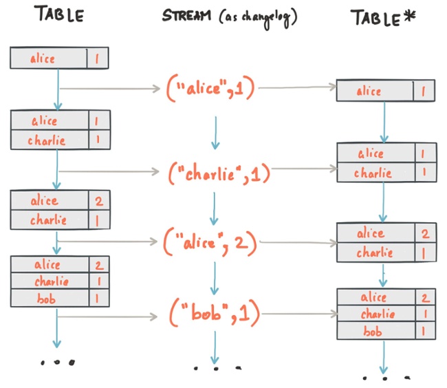 Figure 1: A table is a (changelog) stream is a table is a …
Here, we can capture any mutations to the table — think: INSERT, UPDATE, DELETE statements — into a changelog stream, and then we can reconstruct the exact same table elsewhere from this changelog stream. So tables are just a particular view of a stream! We also realize that a stream can be transformed into a table right away, i.e. without having an “original” table to work from.
Now what is the connection between this abstract concept of a stream-table duality and the practical use case we want to implement? Why should we care?
First, the side data (latest geo-location of users) with which we want to enrich the incoming event stream looks just like such a table in a database: “Alice (key) is currently in Europe (value)”. If we were to capture the geo-locations of our users in a Kafka topic — just like we would do for the incoming stream of user click events — then we could perhaps turn this stream of geo-location changes into a continuously updated table.
Second, and fortunate for us, Kafka Streams ships with built-in support to interpret the data in a Kafka topic as such a continuously updated table. In the Kafka Streams DSL this is achieved via the so-called KTable. More on this later.
Third, and here we are looking a bit behind the scenes of Kafka Streams, these KTables are backed by state stores in Kafka Streams. These state stores are local to your application (more precisely: they are local to the instances of your application, of which there can be one or many), which means that interacting with these state stores does not require talking over the network, so read and write operations are very fast. For the sake of brevity we will not go into the technical details here how state stores are partitioned across the instances of your application to achieve scalability, or how Kafka Streams ensures that these local state stores can be fully recovered in the face of machine failures to prevent data loss (hint: state stores are but tables, and any changes to them can be captured in a changelog stream, which can be persisted to Kafka in log-compacted topics, from which they can be restored).
Now what’s the end result of all this, what have we gained through Kafka Streams? Effectively, the stream-table duality and the concrete implementation of this duality in Kafka Streams provides you with a lightweight embedded “database” that is continuously and transparently updated by Kafka topics. Table data is available locally to the instances of your stream processing application, which means we have achieved data locality for the step of enriching our incoming stream of user click events with the geo-location side data. Lookups against these KTables are very fast so we don’t run into a scalability or latency bottleneck as in the initial scenario of querying an external database. We also achieved isolation, and the availability of our stream processing application is no longer coupled with the availability of an external database. That’s a great fit for these very common stream processing use cases, particularly but not only when you are running at larger scale!
What we want to do
So let’s rebuild this use case properly with a stream processing application that uses Kafka Streams. At a high level our streaming application will perform a join between two input sources:
- The stream of user click events, stored in a Kafka topic. This topic will be read as a KStream using the Kafka Streams DSL.
- The stream of user geo-location updates, stored in another Kafka topic. This topic will be read as a KTable.
The stream of user click events is considered to be a record stream, where each data record represents a self-contained datum. In contrast, the stream of user geo-location updates is interpreted as a changelog stream, where each data record represents an update (i.e. any previous data records having the same record key will be replaced by the latest update). In Kafka Streams, a record stream is represented via the so-called KStream interface and a changelog stream via the KTable interface. Going from the high-level view to the technical view, this means that our streaming application will demonstrate how to perform a join operation between a KStream and a KTable, i.e. it is an example of a stateful computation. This KStream-KTable join also happens to be Kafka Streams’ equivalent of performing a table lookup in a streaming context, where the table is updated continuously and concurrently. Specifically, for each user click event in the KStream, we will lookup the user’s region (e.g. “europe”) in the KTable in order to subsequently compute the total number of user clicks per region.
Let’s showcase the beginning (input) and the end (expected output) of this data pipeline with some example data.
Input stream of user click events:
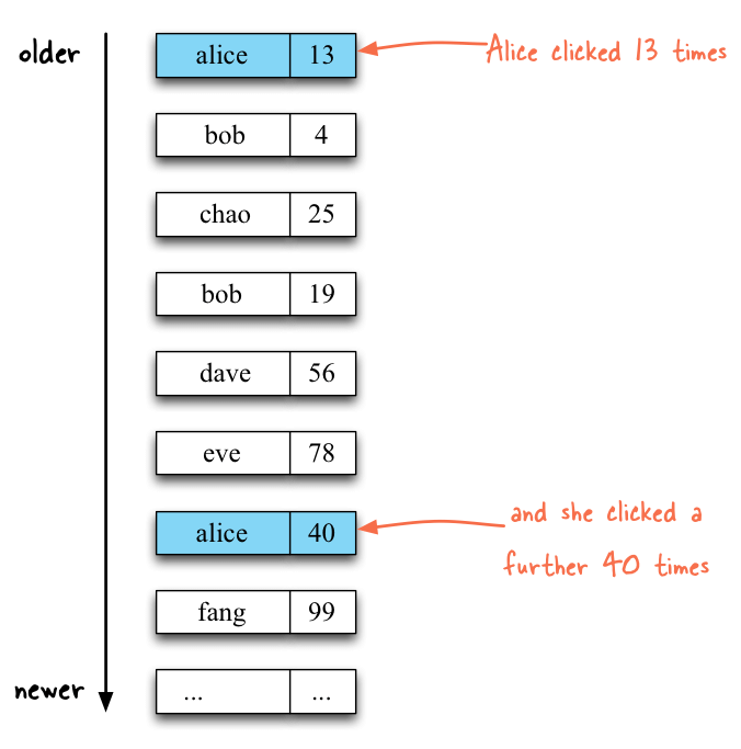
Input stream of user profile updates: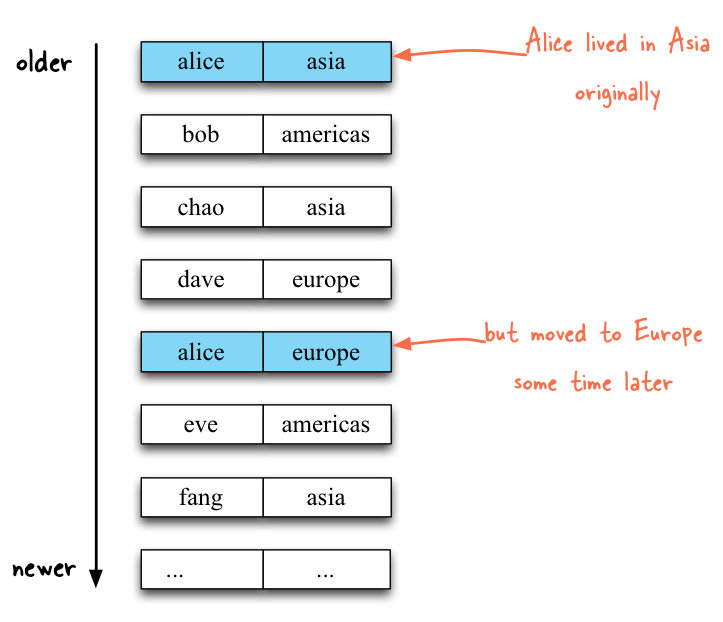
For these input streams we expect a continuously updating table that will track the latest per-region click counts: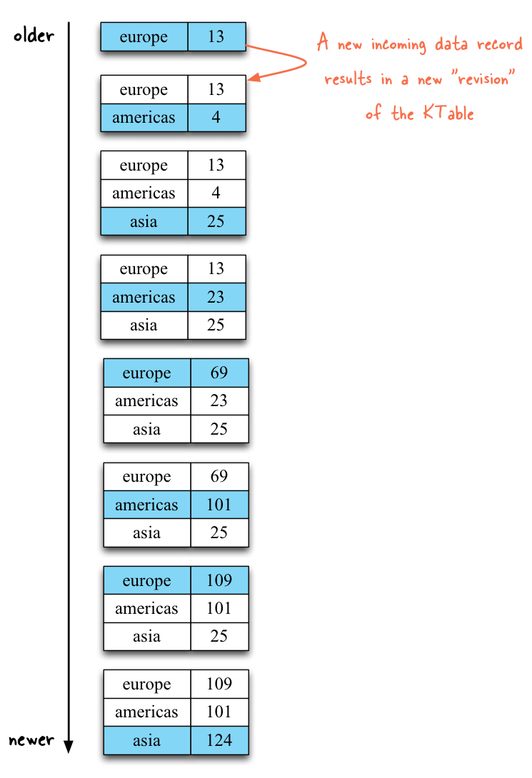
In the next section we will describe how to implement the corresponding data pipeline with Kafka Streams.
Implementation
Overview
The full code of this application is available in the confluentinc/kafka-streams-
In this blog post however let us concentrate on the key parts of the code, which is the definition of the streaming application’s processing topology:
// This KStream contains information such as "alice" -> 13
KStream<String, Long> userClicksStream = builder.stream(..., "user-clicks-topic");// This KTable contains information such as "alice" -> "europe"
KTable<String, String> userRegionsTable = builder.table(..., "user-regions-topic");// Compute the number of clicks per region, e.g. "europe" -> 13
//
// The resulting KTable is continuously being updated as new data records are arriving in the
// input KStream `userClicksStream` and input KTable `userRegionsTable`.
KTable<String, Long> clicksPerRegion = userClicksStream
.leftJoin(userRegionsTable, (clicks, region) -> new RegionWithClicks(region == null ? "UNKNOWN" : region, clicks))
.map((user, regionWithClicks) -> new KeyValue<>(regionWithClicks.getRegion(), regionWithClicks.getClicks()))
.reduceByKey((firstClicks, secondClicks) -> firstClicks + secondClicks, ...);// Write the output back to Kafka so that other applications can use it, too.
clicksPerRegion.to("clicks-per-region-topic", ...);
Reading the input data from Kafka
First we must tell Kafka Streams which input data is being read from Kafka, and how this reading should be performed. Here, we read the “user-clicks-topic” Kafka topic through a KStream instance, i.e. interpret it as a record stream. Secondly, we read the “user-regions-topic” Kafka topic through a KTable instance, i.e. interpret it as a changelog stream. The KTable will allow us to perform fast local table lookups during the upcoming join operation, where we enrich the data in the KStream with side data (user geo-location).
// This KStream contains information such as "alice" -> 13
KStream<String, Long> userClicksStream = builder.stream(..., "user-clicks-topic");
// This KTable contains information such as "alice" -> "europe"
KTable<String, String> userRegionsTable = builder.table(..., "user-regions-topic");
Processing the input data
Now we can define the processing of the input data. The first step of our data pipeline, using leftJoin(), is the aforementioned enriching of the user click events with the latest geo-location of users. In this step we transform the <user, clicks> input stream (of type KStream<String, Long>) to a new <user, (region, clicks)> stream (of type KStream<String, RegionWithClicks>).
userClicksStream.leftJoin(userRegionsTable, (clicks, region) -> new RegionWithClicks(region == null ? "UNKNOWN" : region, clicks))
Because Java doesn’t natively support tuples we must introduce a helper class called RegionWithClicks that tracks the (region, clicks) information. The equivalent Scala application does not need this RegionWithClicks helper class because Scala supports tuples out of the box. Of special note is the null check when creating new RegionWithClicks instances: we must safeguard against table lookup misses, i.e. situations where a username in a user click event is not known or not yet known in the joined KTable. In this particular example, we decide to fall back to a default geo-location value of “UNKNOWN” for such cases.
Here’s an illustration of the stream before and after the join operation.
Before: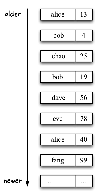
After: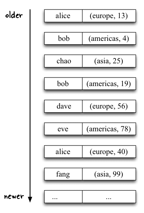
The next step, using map(), is a simple transformation that prepares the final step of summing up the individual number of clicks. The map operator takes a binary function as its input, where the function arguments are the key and the value of the data records in the stream.
map((user, regionWithClicks) -> new KeyValue<>(regionWithClicks.getRegion(), regionWithClicks.getClicks()))
Here, the map step replaces the user as the key of the stream with the region, i.e. it turns the <user, (region, clicks)> stream (of type KStream<String, RegionWithClicks>) into a <region, clicks> stream (of type KStream<String, String>). This preparation step is required because the final transformation, using reduceByKey, operates based on the key of data records; and because we want to compute the total number of clicks per region, the record key must hold the region information.
Here’s an illustration of the stream before and after the map operation.
Before:
After: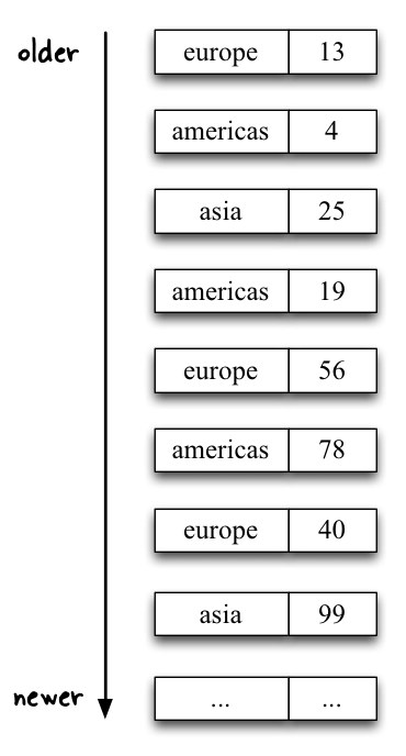
The last step, using reduceByKey(), sums up the individual number of clicks by geo-region. The reduceByKey operator takes a binary function as a parameter, which in our case defines the addition of its two input arguments.
reduceByKey((firstClicks, secondClicks) -> firstClicks + secondClicks, ...)
Note that reduceByKey returns a KTable, i.e. in this step we go from a KStream<String, String> to a KTable<String, Long>. This new KTable tracks the continuously updating <region, totalClicksPerRegion> information that we are interested in.
Here’s an illustration of the stream before and after the reduceByKey operation. Again, note that the result of of the reduceByKey operation is a KTable!
Before (a KStream):
After (now a continuously updating KTable):
As you can see in the output above, the total click counts per region are being updated continuously based on both (a) the newly arriving user click events and (b) newly arriving updates to the user geo-locations. And any such data may arrive concurrently from both sources. For example, if the region of user bob changes from “americas” to “asia” by writing a (“bob”, “asia”) data record to the “user-regions-topic” in Kafka, any (“bob”, numberOfClicks) events that will be received after this geo-location update will then increase the total click count of the “asia” region.
Writing the output data to Kafka
Finally, we can persist the results of these processing steps by writing them back to a Kafka topic, using to():
clicksPerRegion.to("clicks-per-region-topic", ...)
Other streaming applications can then leverage these continuously updating per-region click counts for their own processing needs.
Where to go from here
In this blog post we implemented a very common stream processing use case with Kafka Streams: continuous queries and transformations. We achieved this through only a few lines of code, and the resulting stream processing application is highly scalable and provides low processing latency even for large incoming data volumes.
If you have enjoyed this article, you might want to continue with the following resources to learn more about Apache Kafka’s Streams API:
- Get started with the Kafka Streams API to build your own real-time applications and microservices.
- Walk through our Confluent tutorial for the Kafka Streams API with Docker and play with our Confluent demo applications.
Ist dieser Blog-Beitrag interessant? Jetzt teilen
Confluent-Blog abonnieren
Stop Treating Your LLM Like a Database
GenAI thrives on real-time contextual data: In a modern system, LLMs should be designed to engage, synthesize, and contribute, rather than to simply serve as queryable data stores.
Generative AI Meets Data Streaming (Part III) – Scaling AI in Real Time: Data Streaming and Event-Driven Architecture
In this final part of the blog series, we bring it all together by exploring data streaming platforms (DSPs), event-driven architecture (EDA), and real-time data processing to scale AI-powered solutions across your organization.

